2 Grid-base processing framework of TransBigData
This notebook will introduce the core functions embedded in the Transbigdata package
[1]:
import transbigdata as tbd
import geopandas as gpd
import pandas as pd
import matplotlib.pyplot as plt
import pprint
import random
[2]:
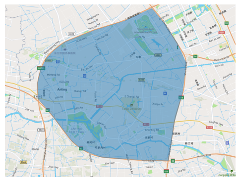
# this is a shp file, the sample area is part of Jiading district, Shanghai, China
jiading_polygon = gpd.read_file(r'data/jiading_polygon/jiading_polygon.shp')
jiading_polygon.head()
[2]:
| id | geometry | |
|---|---|---|
| 0 | 1 | POLYGON ((121.22538 31.35142, 121.22566 31.350... |
[3]:
jiading_rec_bound = [121.1318, 31.2484, 121.2553, 31.3535]

fig = plt.figure(1, (6, 6), dpi=100)
ax = plt.subplot(111)
plt.sca(ax)
tbd.plot_map(plt, bounds=jiading_rec_bound, zoom=13, style=2)

jiading_polygon.plot(ax=ax, alpha=0.5)
plt.axis('off');
transbigdata.area_to_grid(location, accuracy=500, method=’rect’, params=’auto’)
[4]:
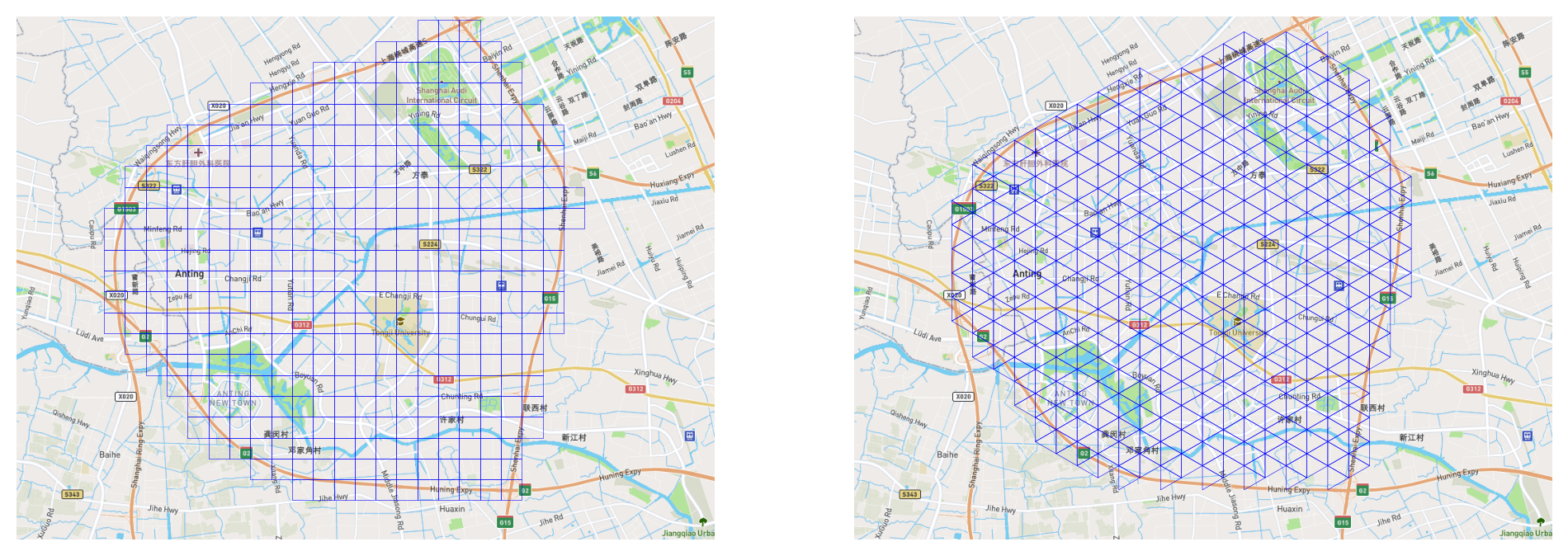
# generate the default grid
grid_rec, params_rec = tbd.area_to_grid(jiading_polygon)
pprint.pprint(params_rec)
grid_rec.head()
{'deltalat': 0.004496605206422906,
 'deltalon': 0.005262604989003139,
 'gridsize': 500,
 'method': 'rect',
 'slat': 31.25168182840957,
 'slon': 121.13797109957756,
 'theta': 0}
[4]:
| LONCOL | LATCOL | geometry | |
|---|---|---|---|
| 171 | 9 | 0 | POLYGON ((121.18270 31.24943, 121.18797 31.249... |
| 174 | 10 | 0 | POLYGON ((121.18797 31.24943, 121.19323 31.249... |
| 177 | 11 | 0 | POLYGON ((121.19323 31.24943, 121.19849 31.249... |
| 180 | 12 | 0 | POLYGON ((121.19849 31.24943, 121.20375 31.249... |
| 183 | 13 | 0 | POLYGON ((121.20375 31.24943, 121.20902 31.249... |
[5]:
# generate triangle grid
grid_tri, params_tri = tbd.area_to_grid(jiading_polygon, method='tri')  # to do: bug need to be fixed here
pprint.pprint(params_tri)
grid_tri.head()
{'deltalat': 0.004496605206422906,
 'deltalon': 0.005262604989003139,
 'gridsize': 500,
 'method': 'tri',
 'slat': 31.25168182840957,
 'slon': 121.13797109957756,
 'theta': 0}
[5]:
| loncol_1 | loncol_2 | loncol_3 | geometry | |
|---|---|---|---|---|
| 22 | 6 | 2 | -5 | POLYGON ((121.17481 31.25947, 121.16955 31.256... |
| 24 | 7 | 2 | -5 | POLYGON ((121.17481 31.25428, 121.18007 31.256... |
| 27 | 8 | 3 | -5 | POLYGON ((121.18007 31.25168, 121.18533 31.254... |
| 28 | 8 | 3 | -6 | POLYGON ((121.18533 31.25947, 121.18007 31.256... |
| 30 | 9 | 3 | -6 | POLYGON ((121.18533 31.25428, 121.19060 31.256... |
[6]:
# Visualization
fig = plt.figure(1, (12, 8), dpi=200)
ax1 = plt.subplot(121)
plt.sca(ax1)
tbd.plot_map(plt, bounds=jiading_rec_bound, zoom=13, style=2)
grid_rec.plot(ax=ax1, lw=0.2, edgecolor='blue', facecolor="None")

plt.axis('off');

ax2 = plt.subplot(122)
plt.sca(ax2)
tbd.plot_map(plt, bounds=jiading_rec_bound, zoom=13, style=2)
grid_tri.plot(ax=ax2, lw=0.2, edgecolor='blue', facecolor="None")

plt.axis('off');
transbigdata.area_to_params(location, accuracy=500, method=’rect’)
Sometime, due to data sparisity, we do not need to generate all the grids. In such case, we can use transbigdata.area_to_params.
This method only creat a dictionary file for the grid, thus is much faster.
[7]:
params = tbd.area_to_params(jiading_polygon)
pprint.pprint(params)
{'deltalat': 0.004496605206422906,
 'deltalon': 0.005262604989003139,
 'gridsize': 500,
 'method': 'rect',
 'slat': 31.25168182840957,
 'slon': 121.13797109957756,
 'theta': 0}
transbigdata.GPS_to_grid(lon, lat, params)
The next common step is to know which grid does each trajectory point belong to.
[8]:
# First, we generate some random GPS points (20 points in this case)

lon_list, lat_list = [], []
for i in range(20):
    gps_lon = random.uniform(jiading_rec_bound[0], jiading_rec_bound[2])
    gps_lat = random.uniform(jiading_rec_bound[1], jiading_rec_bound[3])
    lon_list.append(gps_lon)
    lat_list.append(gps_lat)

gps_random = pd.DataFrame({'veh_id': range(20),
                           'lon': lon_list,
                           'lat': lat_list,
                          })

gps_random.head()
[8]:
| veh_id | lon | lat | |
|---|---|---|---|
| 0 | 0 | 121.204726 | 31.266296 |
| 1 | 1 | 121.168077 | 31.326952 |
| 2 | 2 | 121.142706 | 31.315498 |
| 3 | 3 | 121.215899 | 31.339561 |
| 4 | 4 | 121.217937 | 31.269540 |
[9]:
# match each point to the rect grid
gps_random['LonCol'], gps_random['LatCol'] = tbd.GPS_to_grid(gps_random['lon'], gps_random['lat'], params_rec)

gps_random.head()
[9]:
| veh_id | lon | lat | LonCol | LatCol | |
|---|---|---|---|---|---|
| 0 | 0 | 121.204726 | 31.266296 | 13 | 3 |
| 1 | 1 | 121.168077 | 31.326952 | 6 | 17 |
| 2 | 2 | 121.142706 | 31.315498 | 1 | 14 |
| 3 | 3 | 121.215899 | 31.339561 | 15 | 20 |
| 4 | 4 | 121.217937 | 31.269540 | 15 | 4 |
transbigdata.grid_to_centre(gridid, params)
The center location of each grid can acquired using transbigdata.grid_to_centre
[10]:
# Use the matched grid as example
gps_random['LonGridCenter'], gps_random['LatGridCenter'] = \
tbd.grid_to_centre([gps_random['LonCol'], gps_random['LatCol']], params_rec)

# check the matched results
gps_random.head()
[10]:
| veh_id | lon | lat | LonCol | LatCol | LonGridCenter | LatGridCenter | |
|---|---|---|---|---|---|---|---|
| 0 | 0 | 121.204726 | 31.266296 | 13 | 3 | 121.206385 | 31.265172 |
| 1 | 1 | 121.168077 | 31.326952 | 6 | 17 | 121.169547 | 31.328124 |
| 2 | 2 | 121.142706 | 31.315498 | 1 | 14 | 121.143234 | 31.314634 |
| 3 | 3 | 121.215899 | 31.339561 | 15 | 20 | 121.216910 | 31.341614 |
| 4 | 4 | 121.217937 | 31.269540 | 15 | 4 | 121.216910 | 31.269668 |
transbigdata.grid_to_polygon(gridid, params)
For visualization convenience, grid parameters can be transformed into geometry format
[11]:
# Use the matched grid as example again
gps_random['grid_geo_polygon'] = tbd.grid_to_polygon([gps_random['LonCol'], gps_random['LatCol']], params_rec)

# check the matched results
gps_random.head()
[11]:
| veh_id | lon | lat | LonCol | LatCol | LonGridCenter | LatGridCenter | grid_geo_polygon | |
|---|---|---|---|---|---|---|---|---|
| 0 | 0 | 121.204726 | 31.266296 | 13 | 3 | 121.206385 | 31.265172 | POLYGON ((121.2037536619401 31.262923341425626... |
| 1 | 1 | 121.168077 | 31.326952 | 6 | 17 | 121.169547 | 31.328124 | POLYGON ((121.16691542701707 31.32587581431555... |
| 2 | 2 | 121.142706 | 31.315498 | 1 | 14 | 121.143234 | 31.314634 | POLYGON ((121.14060240207206 31.31238599869628... |
| 3 | 3 | 121.215899 | 31.339561 | 15 | 20 | 121.216910 | 31.341614 | POLYGON ((121.2142788719181 31.339365629934818... |
| 4 | 4 | 121.217937 | 31.269540 | 15 | 4 | 121.216910 | 31.269668 | POLYGON ((121.2142788719181 31.26741994663205,... |
transbigdata.grid_to_area(data, shape, params, col=[‘LONCOL’, ‘LATCOL’])
In addition to grid, there might be several districts. transbigdata.grid_to_area can be used to match the information.
In this case, there are only one district in jiading_polygon, the matched column is id.
[12]:
gps_matched = tbd.grid_to_area(gps_random, jiading_polygon, params_rec, col=['LonCol', 'LatCol'])

# check the matched results
gps_matched.head()
/Applications/anaconda3/envs/tbd/lib/python3.9/site-packages/transbigdata/grids.py:421: UserWarning: CRS mismatch between the CRS of left geometries and the CRS of right geometries.
Use `to_crs()` to reproject one of the input geometries to match the CRS of the other.

Left CRS: None
Right CRS: EPSG:4326

  data1 = gpd.sjoin(data1, shape)
[12]:
| veh_id | lon | lat | LonCol | LatCol | LonGridCenter | LatGridCenter | grid_geo_polygon | geometry | index_right | id | |
|---|---|---|---|---|---|---|---|---|---|---|---|
| 0 | 0 | 121.204726 | 31.266296 | 13 | 3 | 121.206385 | 31.265172 | POLYGON ((121.2037536619401 31.262923341425626... | POINT (121.20638 31.26517) | 0 | 1 |
| 1 | 1 | 121.168077 | 31.326952 | 6 | 17 | 121.169547 | 31.328124 | POLYGON ((121.16691542701707 31.32587581431555... | POINT (121.16955 31.32812) | 0 | 1 |
| 2 | 2 | 121.142706 | 31.315498 | 1 | 14 | 121.143234 | 31.314634 | POLYGON ((121.14060240207206 31.31238599869628... | POINT (121.14323 31.31463) | 0 | 1 |
| 3 | 3 | 121.215899 | 31.339561 | 15 | 20 | 121.216910 | 31.341614 | POLYGON ((121.2142788719181 31.339365629934818... | POINT (121.21691 31.34161) | 0 | 1 |
| 4 | 4 | 121.217937 | 31.269540 | 15 | 4 | 121.216910 | 31.269668 | POLYGON ((121.2142788719181 31.26741994663205,... | POINT (121.21691 31.26967) | 0 | 1 |
transbigdata.grid_to_params(grid)
A useful tool to get grid params from grid geometry
[13]:
# this is the formal grid geometry
grid_rec.head()
[13]:
| LONCOL | LATCOL | geometry | |
|---|---|---|---|
| 171 | 9 | 0 | POLYGON ((121.18270 31.24943, 121.18797 31.249... |
| 174 | 10 | 0 | POLYGON ((121.18797 31.24943, 121.19323 31.249... |
| 177 | 11 | 0 | POLYGON ((121.19323 31.24943, 121.19849 31.249... |
| 180 | 12 | 0 | POLYGON ((121.19849 31.24943, 121.20375 31.249... |
| 183 | 13 | 0 | POLYGON ((121.20375 31.24943, 121.20902 31.249... |
[14]:
tbd.grid_to_params(grid_rec)
[14]:
{'slon': 121.13797109957761,
 'slat': 31.25168182840957,
 'deltalon': 0.005262604988999442,
 'deltalat': 0.0044966052064197015,
 'theta': 0,
 'method': 'rect'}
transbigdata.grid_params_optimize(data, initialparams, col=[‘uid’, ‘lon’, ‘lat’], optmethod=’centerdist’, printlog=False, sample=0)
Offers several methods to optimize the grids
This method relies on the scikit-opt package. To do so, please run following code in cmd:
pip install scikit-opt
For more details of this method, please refer to this notebook.
[15]:
# we use the random generated data again
gps_random.head()
[15]:
| veh_id | lon | lat | LonCol | LatCol | LonGridCenter | LatGridCenter | grid_geo_polygon | |
|---|---|---|---|---|---|---|---|---|
| 0 | 0 | 121.204726 | 31.266296 | 13 | 3 | 121.206385 | 31.265172 | POLYGON ((121.2037536619401 31.262923341425626... |
| 1 | 1 | 121.168077 | 31.326952 | 6 | 17 | 121.169547 | 31.328124 | POLYGON ((121.16691542701707 31.32587581431555... |
| 2 | 2 | 121.142706 | 31.315498 | 1 | 14 | 121.143234 | 31.314634 | POLYGON ((121.14060240207206 31.31238599869628... |
| 3 | 3 | 121.215899 | 31.339561 | 15 | 20 | 121.216910 | 31.341614 | POLYGON ((121.2142788719181 31.339365629934818... |
| 4 | 4 | 121.217937 | 31.269540 | 15 | 4 | 121.216910 | 31.269668 | POLYGON ((121.2142788719181 31.26741994663205,... |
[16]:
tbd.grid_params_optimize(gps_random, params_rec, col=['veh_id', 'lon', 'lat'],printlog=True)
Optimized index centerdist: 116.11243965546235
Optimized gridding params: {'slon': 121.14169760115118, 'slat': 31.252579076220087, 'deltalon': 0.005262604989003139, 'deltalat': 0.004496605206422906, 'theta': 50.91831009508256, 'method': 'rect'}
Optimizing cost:
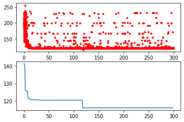
Result:

[16]:
{'slon': 121.14169760115118,
 'slat': 31.252579076220087,
 'deltalon': 0.005262604989003139,
 'deltalat': 0.004496605206422906,
 'theta': 50.91831009508256,
 'method': 'rect'}