1 Processing & visualizing taxi GPS data
Taxi GPS data processing
[1]:
import transbigdata as tbd
import pandas as pd
import geopandas as gpd
import matplotlib.pyplot as plt

# Read data
data = pd.read_csv('data/TaxiData-Sample.csv', header=None)
data.columns = ['VehicleNum', 'Time', 'Lng', 'Lat', 'OpenStatus', 'Speed']
data.head()
[1]:
| VehicleNum | Time | Lng | Lat | OpenStatus | Speed | |
|---|---|---|---|---|---|---|
| 0 | 34745 | 20:27:43 | 113.806847 | 22.623249 | 1 | 27 |
| 1 | 34745 | 20:24:07 | 113.809898 | 22.627399 | 0 | 0 |
| 2 | 34745 | 20:24:27 | 113.809898 | 22.627399 | 0 | 0 |
| 3 | 34745 | 20:22:07 | 113.811348 | 22.628067 | 0 | 0 |
| 4 | 34745 | 20:10:06 | 113.819885 | 22.647800 | 0 | 54 |
[2]:
# Read the GeoDataFrame of the study area
sz = gpd.read_file(r'data/sz.json')
sz.crs = None
sz.head()
[2]:
| centroid_x | centroid_y | qh | geometry | |
|---|---|---|---|---|
| 0 | 114.143157 | 22.577605 | 罗湖 | POLYGON ((114.10006 22.53431, 114.10083 22.534... |
| 1 | 114.041535 | 22.546180 | 福田 | POLYGON ((113.98578 22.51348, 114.00553 22.513... |
| 2 | 114.270206 | 22.596432 | 盐田 | POLYGON ((114.19799 22.55673, 114.19817 22.556... |
| 3 | 113.851387 | 22.679120 | 宝安 | MULTIPOLYGON (((113.81831 22.54676, 113.81948 ... |
| 4 | 113.926290 | 22.766157 | 光明 | POLYGON ((113.99768 22.76643, 113.99704 22.766... |
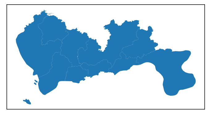
[3]:
fig = plt.figure(1, (8, 3), dpi=150)
ax1 = plt.subplot(111)
sz.plot(ax=ax1)
plt.xticks([], fontsize=10)
plt.yticks([], fontsize=10);
Data pre-processing
TransBigData integrates several common methods for data pre-processing. Using the tbd.clean_outofshape method, given the data and the GeoDataFrame of the study area, it can delete the data outside the study area. The tbd.clean_taxi_status method can filters out the data with instantaneous changes in passenger status(OpenStatus). When using the preprocessing method, the corresponding column names need to be passed in as parameters:
[4]:
# Data Preprocessing
# Delete the data outside of the study area
data = tbd.clean_outofshape(data, sz, col=['Lng', 'Lat'], accuracy=500)

# Delete the data with instantaneous changes in passenger status
data = tbd.clean_taxi_status(data, col=['VehicleNum', 'Time', 'OpenStatus'])
Data Gridding
The most basic way to express the data distribution is in the form of geograpic grids; after the data gridding, each GPS data point is mapped to the corresponding grid. For data gridding, you need to determine the gridding parameters at first(which can be interpreted as defining a grid coordinate system):
[5]:
# Data gridding
# Define the bounds and generate gridding parameters
bounds = [113.6, 22.4, 114.8, 22.9]
params = tbd.area_to_params(bounds, accuracy=500)
print(params)
{'slon': 113.6, 'slat': 22.4, 'deltalon': 0.004872390756896538, 'deltalat': 0.004496605206422906, 'theta': 0, 'method': 'rect', 'gridsize': 500}
After obtaining the gridding parameters, the next step is to map the GPS is to their corresponding grids. Using the tbd.GPS_to_grids, it will generate the LONCOL column and the LATCOL column. The two columns together can specify a grid:
[6]:
# Mapping GPS data to grids
data['LONCOL'], data['LATCOL'] = tbd.GPS_to_grid(data['Lng'], data['Lat'], params)
data.head()
[6]:
| VehicleNum | Time | Lng | Lat | OpenStatus | Speed | LONCOL | LATCOL | |
|---|---|---|---|---|---|---|---|---|
| 0 | 34745 | 20:27:43 | 113.806847 | 22.623249 | 1 | 27 | 42 | 50 |
| 1 | 27368 | 09:08:53 | 113.805893 | 22.624996 | 0 | 49 | 42 | 50 |
| 2 | 22998 | 10:51:10 | 113.806931 | 22.624166 | 1 | 54 | 42 | 50 |
| 3 | 22998 | 10:11:50 | 113.805946 | 22.625433 | 0 | 43 | 42 | 50 |
| 4 | 22998 | 10:12:05 | 113.806381 | 22.623833 | 0 | 60 | 42 | 50 |
Count the amount of data in each grids:
[7]:
# Aggregate data into grids
datatest = data.groupby(['LONCOL', 'LATCOL'])['VehicleNum'].count().reset_index()
datatest.head()
[7]:
| LONCOL | LATCOL | VehicleNum | |
|---|---|---|---|
| 0 | 36 | 63 | 2 |
| 1 | 36 | 66 | 1 |
| 2 | 36 | 67 | 8 |
| 3 | 37 | 62 | 9 |
| 4 | 37 | 63 | 8 |
Generate the geometry of the grids and transform it into a GeoDataFrame:
[8]:
# Generate the geometry for grids
datatest['geometry'] = tbd.grid_to_polygon([datatest['LONCOL'], datatest['LATCOL']], params)

# Change it into GeoDataFrame
# import geopandas as gpd
datatest = gpd.GeoDataFrame(datatest)
datatest.head()
[8]:
| LONCOL | LATCOL | VehicleNum | geometry | |
|---|---|---|---|---|
| 0 | 36 | 63 | 2 | POLYGON ((113.77297 22.68104, 113.77784 22.681... |
| 1 | 36 | 66 | 1 | POLYGON ((113.77297 22.69453, 113.77784 22.694... |
| 2 | 36 | 67 | 8 | POLYGON ((113.77297 22.69902, 113.77784 22.699... |
| 3 | 37 | 62 | 9 | POLYGON ((113.77784 22.67654, 113.78271 22.676... |
| 4 | 37 | 63 | 8 | POLYGON ((113.77784 22.68104, 113.78271 22.681... |
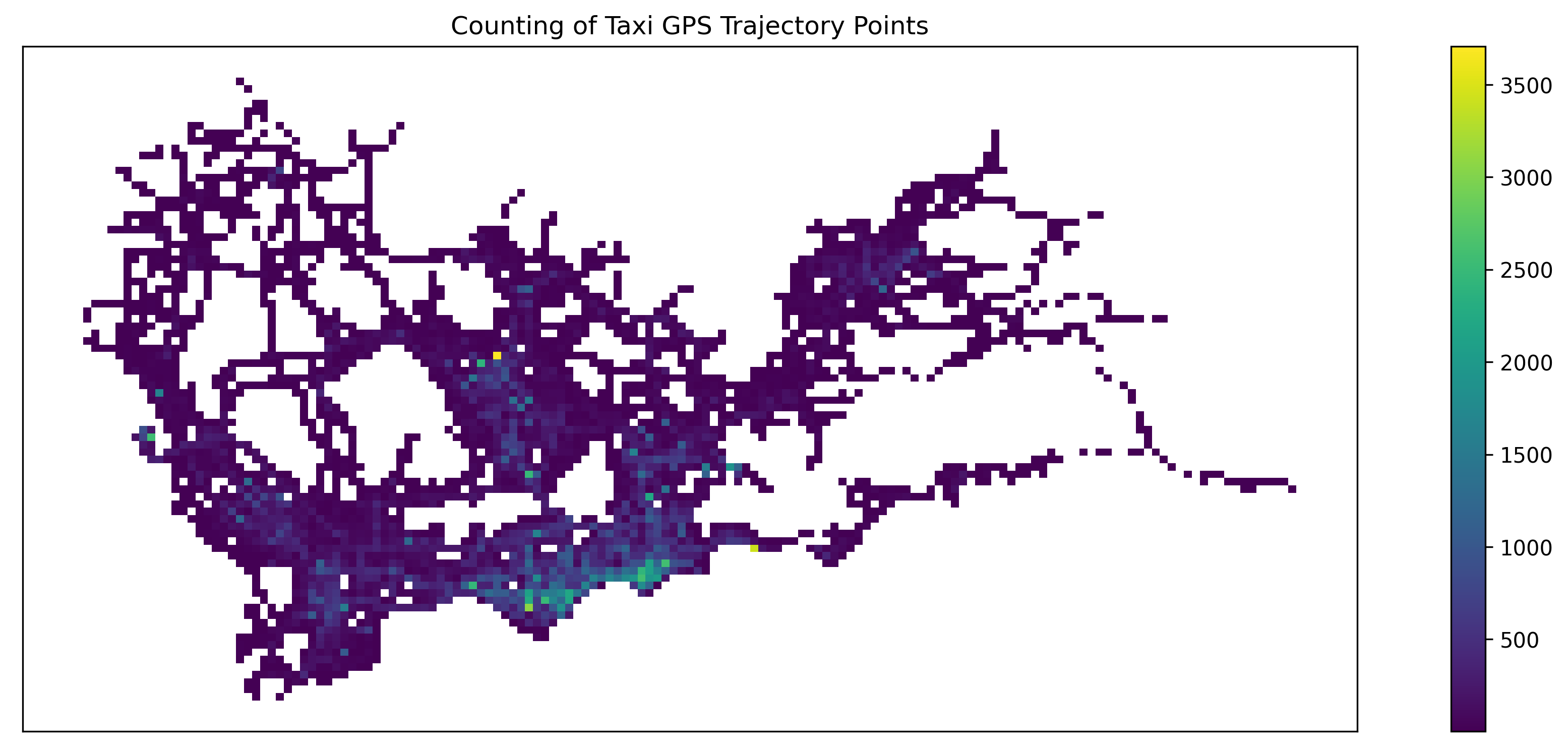
Plot the generated grids:
[9]:
# Plot the grids
fig = plt.figure(1, (16, 6), dpi=300)
ax1 = plt.subplot(111)

# tbd.plot_map(plt, bounds, zoom=10, style=4)
datatest.plot(ax=ax1, column='VehicleNum', legend=True)
plt.xticks([], fontsize=10)
plt.yticks([], fontsize=10)
plt.title('Counting of Taxi GPS Trajectory Points', fontsize=12);
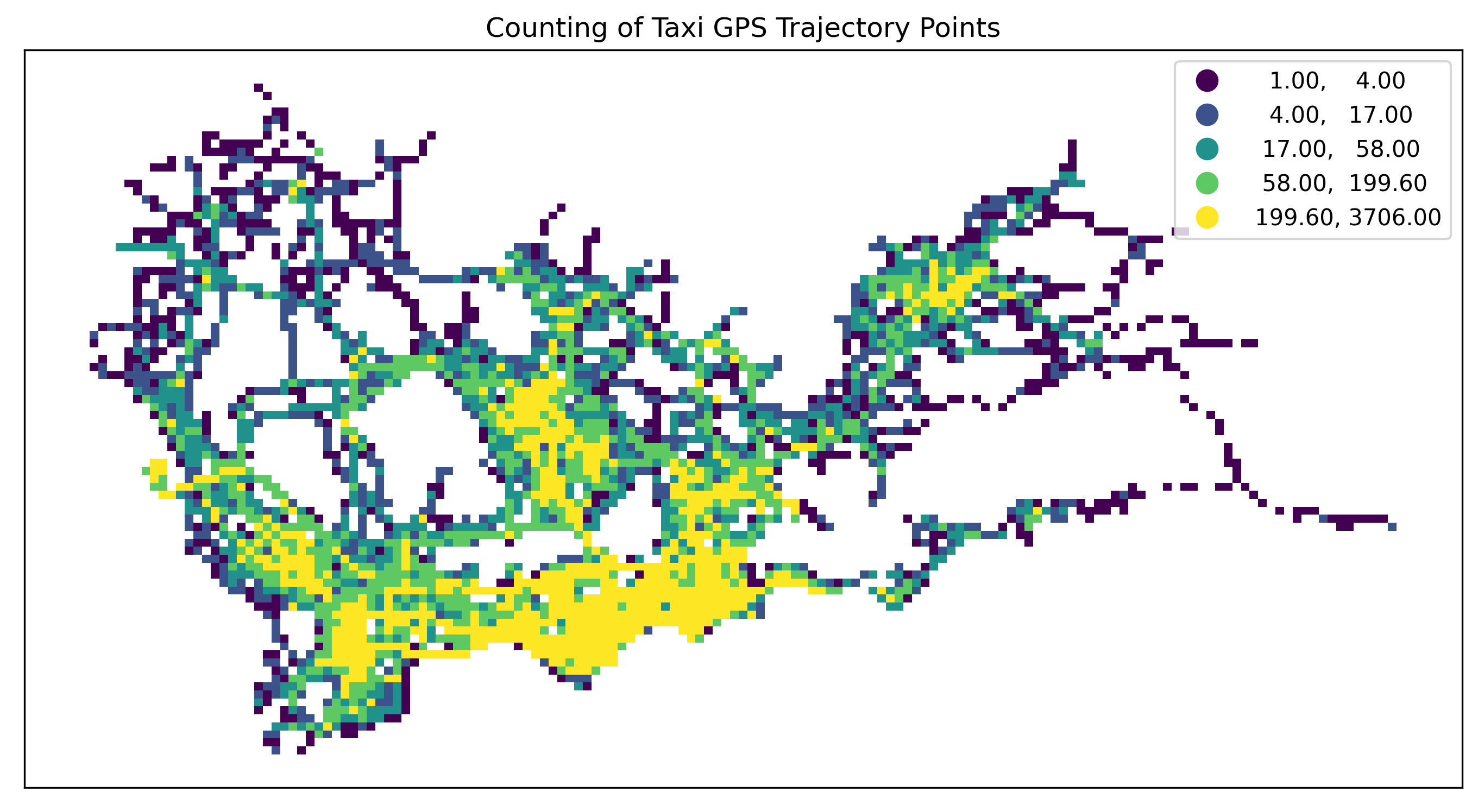
[10]:
# Plot the grids
fig = plt.figure(1, (16, 6), dpi=300) # 确定图形高为6,宽为8;图形清晰度
ax1 = plt.subplot(111)
datatest.plot(ax=ax1, column='VehicleNum', legend=True, scheme='quantiles')
# plt.legend(fontsize=10)
plt.xticks([], fontsize=10)
plt.yticks([], fontsize=10)
plt.title('Counting of Taxi GPS Trajectory Points', fontsize=12);
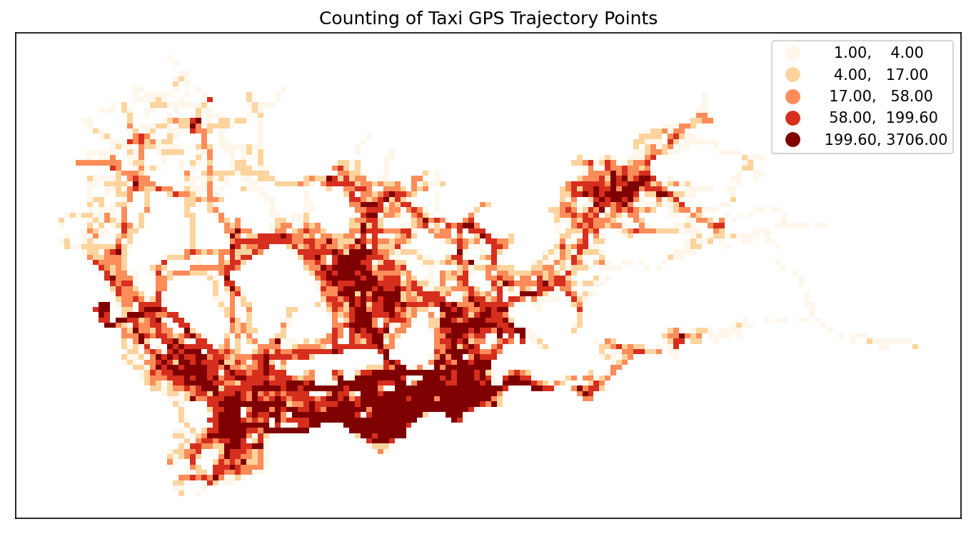
[11]:
# Plot the grids
fig = plt.figure(1, (16, 6), dpi=150) # 确定图形高为6,宽为8;图形清晰度
ax1 = plt.subplot(111)
datatest.plot(ax=ax1, column='VehicleNum', legend=True, cmap='OrRd', scheme='quantiles')
# plt.legend(fontsize=10)
plt.xticks([], fontsize=10)
plt.yticks([], fontsize=10)
plt.title('Counting of Taxi GPS Trajectory Points', fontsize=12);
Origin-destination(OD) Extraction and aggregate taxi trips
Use the tbd.taxigps_to_od method and pass in the corresponding column name to extract the taxi trip OD:
[12]:
# Extract taxi OD from GPS data
oddata = tbd.taxigps_to_od(data,col = ['VehicleNum', 'Time', 'Lng', 'Lat', 'OpenStatus'])
oddata
[12]:
| VehicleNum | stime | slon | slat | etime | elon | elat | ID | |
|---|---|---|---|---|---|---|---|---|
| 427075 | 22396 | 00:19:41 | 114.013016 | 22.664818 | 00:23:01 | 114.021400 | 22.663918 | 0 |
| 131301 | 22396 | 00:41:51 | 114.021767 | 22.640200 | 00:43:44 | 114.026070 | 22.640266 | 1 |
| 417417 | 22396 | 00:45:44 | 114.028099 | 22.645082 | 00:47:44 | 114.030380 | 22.650017 | 2 |
| 376160 | 22396 | 01:08:26 | 114.034897 | 22.616301 | 01:16:34 | 114.035614 | 22.646717 | 3 |
| 21768 | 22396 | 01:26:06 | 114.046021 | 22.641251 | 01:34:48 | 114.066048 | 22.636183 | 4 |
| ... | ... | ... | ... | ... | ... | ... | ... | ... |
| 57666 | 36805 | 22:37:42 | 114.113403 | 22.534767 | 22:48:01 | 114.114365 | 22.550632 | 5332 |
| 175519 | 36805 | 22:49:12 | 114.114365 | 22.550632 | 22:50:40 | 114.115501 | 22.557983 | 5333 |
| 212092 | 36805 | 22:52:07 | 114.115402 | 22.558083 | 23:03:27 | 114.118484 | 22.547867 | 5334 |
| 119041 | 36805 | 23:03:45 | 114.118484 | 22.547867 | 23:20:09 | 114.133286 | 22.617750 | 5335 |
| 224103 | 36805 | 23:36:19 | 114.112968 | 22.549601 | 23:43:12 | 114.089485 | 22.538918 | 5336 |
5337 rows × 8 columns
Aggregate the extracted OD and generate LineString GeoDataFrame
[13]:
# Gridding and aggragate data
od_gdf = tbd.odagg_grid(oddata, params)
od_gdf.head()
/opt/anaconda3/lib/python3.8/site-packages/pandas/core/dtypes/cast.py:91: ShapelyDeprecationWarning: The array interface is deprecated and will no longer work in Shapely 2.0. Convert the '.coords' to a numpy array instead.
  values = construct_1d_object_array_from_listlike(values)
[13]:
| SLONCOL | SLATCOL | ELONCOL | ELATCOL | count | SHBLON | SHBLAT | EHBLON | EHBLAT | geometry | |
|---|---|---|---|---|---|---|---|---|---|---|
| 0 | 40 | 62 | 45 | 68 | 1 | 113.794896 | 22.678790 | 113.819258 | 22.705769 | LINESTRING (113.79490 22.67879, 113.81926 22.7... |
| 3331 | 101 | 36 | 86 | 29 | 1 | 114.092111 | 22.561878 | 114.019026 | 22.530402 | LINESTRING (114.09211 22.56188, 114.01903 22.5... |
| 3330 | 101 | 35 | 105 | 30 | 1 | 114.092111 | 22.557381 | 114.111601 | 22.534898 | LINESTRING (114.09211 22.55738, 114.11160 22.5... |
| 3329 | 101 | 34 | 109 | 34 | 1 | 114.092111 | 22.552885 | 114.131091 | 22.552885 | LINESTRING (114.09211 22.55288, 114.13109 22.5... |
| 3328 | 101 | 34 | 103 | 34 | 1 | 114.092111 | 22.552885 | 114.101856 | 22.552885 | LINESTRING (114.09211 22.55288, 114.10186 22.5... |
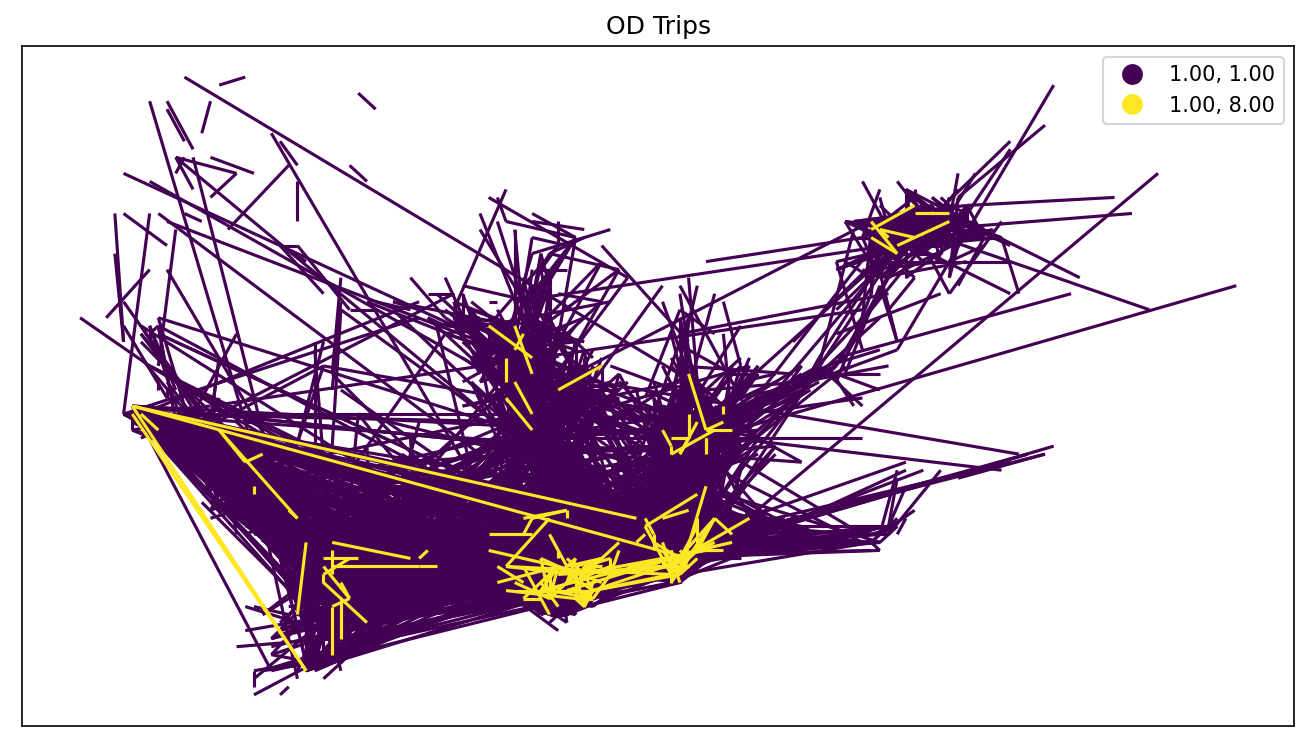
[14]:
# Plot the grids
fig = plt.figure(1, (16, 6), dpi=150) # 确定图形高为6,宽为8;图形清晰度
ax1 = plt.subplot(111)
# data_grid_count.plot(ax=ax1, column='VehicleNum', legend=True, cmap='OrRd', scheme='quantiles')

od_gdf.plot(ax=ax1, column='count', legend=True, scheme='quantiles')
plt.xticks([], fontsize=10)
plt.yticks([], fontsize=10)
plt.title('OD Trips', fontsize=12);
/opt/anaconda3/lib/python3.8/site-packages/mapclassify/classifiers.py:238: UserWarning: Warning: Not enough unique values in array to form k classes
  Warn(
/opt/anaconda3/lib/python3.8/site-packages/mapclassify/classifiers.py:241: UserWarning: Warning: setting k to 2
  Warn("Warning: setting k to %d" % k_q, UserWarning)
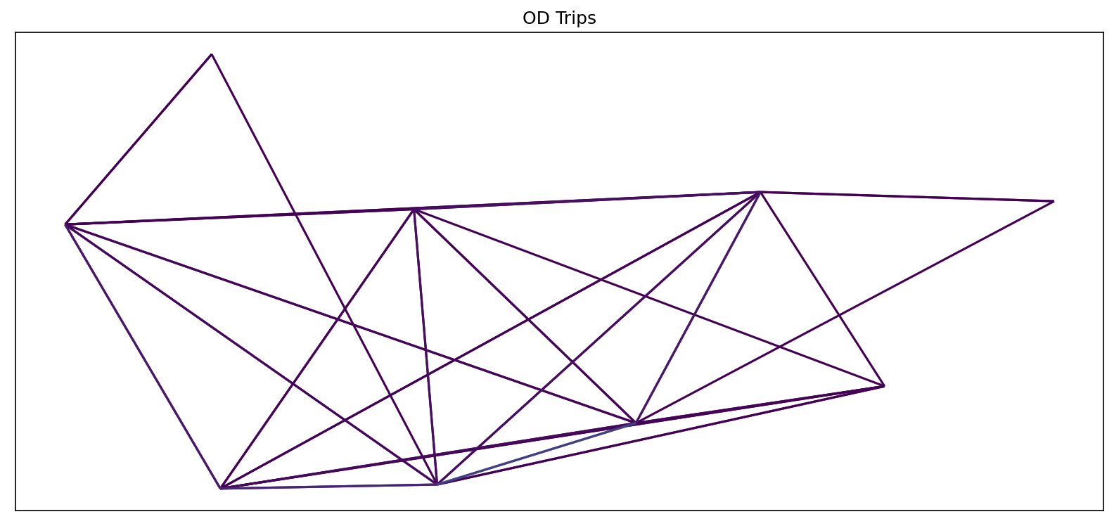
Aggregate OD into polygons
TransBigData also provides the method for aggregating OD into polygons
[15]:
# Aggragate OD data to polygons
# without passing gridding parameters, the algorithm will map the data
# to polygons directly using their coordinates
od_gdf = tbd.odagg_shape(oddata, sz, round_accuracy=6)
fig = plt.figure(1, (16, 6), dpi=150) # 确定图形高为6,宽为8;图形清晰度
ax1 = plt.subplot(111)
od_gdf.plot(ax=ax1, column='count')
plt.xticks([], fontsize=10)
plt.yticks([], fontsize=10)
plt.title('OD Trips', fontsize=12);
/opt/anaconda3/lib/python3.8/site-packages/pandas/core/dtypes/cast.py:91: ShapelyDeprecationWarning: The array interface is deprecated and will no longer work in Shapely 2.0. Convert the '.coords' to a numpy array instead.
  values = construct_1d_object_array_from_listlike(values)
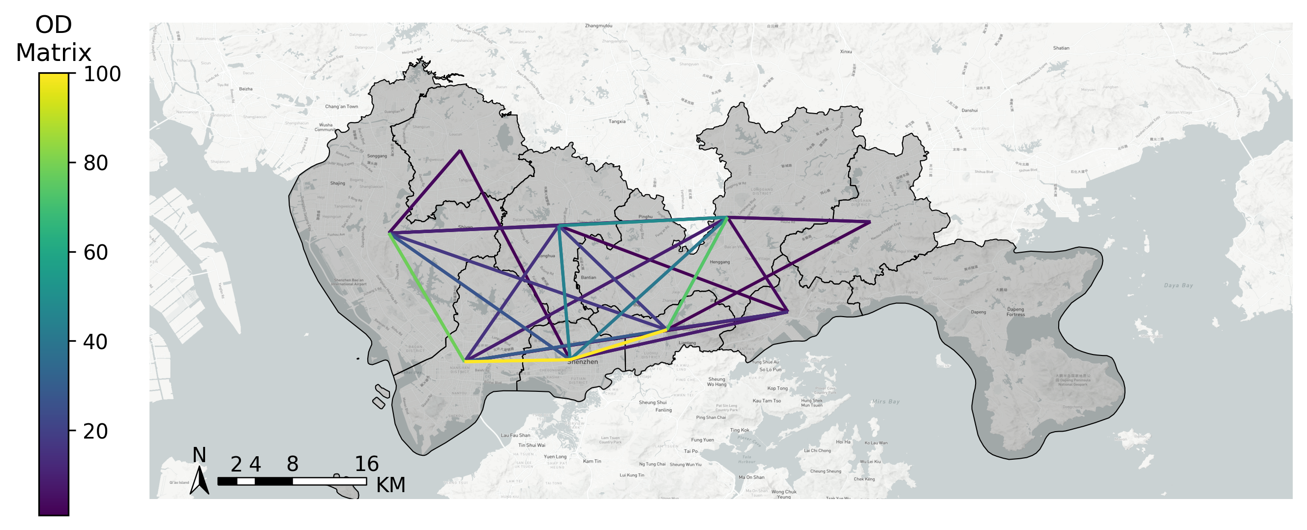
Matplotlib-based map drawing
TransBigData also provide basemap loading in matplotlib. Before using this method, you need to set your mapboxtoken and the storage location for the basemap, see: this link。tbd.plot_map to add basemap and tbd.plotscale to add scale and compass:
[16]:
# Create figure
fig = plt.figure(1, (10, 10), dpi=300)
ax = plt.subplot(111)
plt.sca(ax)

# Load basemap
tbd.plot_map(plt, bounds, zoom=12, style=4)

# Define an ax for colorbar
cax = plt.axes([0.05, 0.33, 0.02, 0.3])
plt.title('OD\nMatrix')
plt.sca(ax)

# Plot the OD
od_gdf.plot(ax=ax, vmax=100, column='count', cax=cax, legend=True)

# Plot the polygons
sz.plot(ax=ax, edgecolor=(0, 0, 0, 1), facecolor=(0, 0, 0, 0.2), linewidths=0.5)

# Add compass and scale
tbd.plotscale(ax, bounds=bounds, textsize=10, compasssize=1, accuracy=2000, rect=[0.06, 0.03], zorder=10)
plt.axis('off')
plt.xlim(bounds[0], bounds[2])
plt.ylim(bounds[1], bounds[3])
plt.show()
Extraction of taxi trajectpries
Using tbd.taxigps_traj_point method, inputing GPS data and OD data, trajectory points can be extracted
[17]:
data_deliver, data_idle = tbd.taxigps_traj_point(data,oddata,col=['VehicleNum',
                                                                  'Time',
                                                                  'Lng',
                                                                  'Lat',
                                                                  'OpenStatus'])
[18]:
data_deliver.head()
[18]:
| VehicleNum | Time | Lng | Lat | OpenStatus | Speed | LONCOL | LATCOL | ID | flag | |
|---|---|---|---|---|---|---|---|---|---|---|
| 427075 | 22396 | 00:19:41 | 114.013016 | 22.664818 | 1 | 63.0 | 85.0 | 59.0 | 0.0 | 1.0 |
| 427085 | 22396 | 00:19:49 | 114.014030 | 22.665483 | 1 | 55.0 | 85.0 | 59.0 | 0.0 | 1.0 |
| 416622 | 22396 | 00:21:01 | 114.018898 | 22.662500 | 1 | 1.0 | 86.0 | 58.0 | 0.0 | 1.0 |
| 427480 | 22396 | 00:21:41 | 114.019348 | 22.662300 | 1 | 7.0 | 86.0 | 58.0 | 0.0 | 1.0 |
| 416623 | 22396 | 00:22:21 | 114.020615 | 22.663366 | 1 | 0.0 | 86.0 | 59.0 | 0.0 | 1.0 |
[19]:
data_idle.head()
[19]:
| VehicleNum | Time | Lng | Lat | OpenStatus | Speed | LONCOL | LATCOL | ID | flag | |
|---|---|---|---|---|---|---|---|---|---|---|
| 416628 | 22396 | 00:23:01 | 114.021400 | 22.663918 | 0 | 25.0 | 86.0 | 59.0 | 0.0 | 0.0 |
| 401744 | 22396 | 00:25:01 | 114.027115 | 22.662100 | 0 | 25.0 | 88.0 | 58.0 | 0.0 | 0.0 |
| 394630 | 22396 | 00:25:41 | 114.024551 | 22.659834 | 0 | 21.0 | 87.0 | 58.0 | 0.0 | 0.0 |
| 394671 | 22396 | 00:26:21 | 114.022797 | 22.658367 | 0 | 0.0 | 87.0 | 57.0 | 0.0 | 0.0 |
| 394672 | 22396 | 00:26:29 | 114.022797 | 22.658367 | 0 | 0.0 | 87.0 | 57.0 | 0.0 | 0.0 |
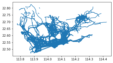
Generate delivery and idle trajectories from trajectory points
[20]:
traj_deliver = tbd.points_to_traj(data_deliver)
traj_deliver.plot();
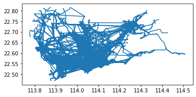
[21]:
traj_idle = tbd.points_to_traj(data_idle[data_idle['OpenStatus'] == 0])
traj_idle.plot()
[21]:
<AxesSubplot:>
Trajectories visualization
Built-in visualization capabilities of TransBigData leverage the visualization package keplergl to interactively visualize data on Jupyter notebook with simple code. To use this method, please install the keplergl package for python:
pip install keplergl
Detailed information please see this link
Visualization of trajectory data:
[22]:
tbd.visualization_trip(data_deliver)
Processing trajectory data...
Generate visualization...
User Guide: https://docs.kepler.gl/docs/keplergl-jupyter