1 出租车GPS数据处理与可视化
出租车GPS数据处理
[1]:
import transbigdata as tbd
import pandas as pd
import geopandas as gpd
import matplotlib.pyplot as plt

# Read data
data = pd.read_csv('data/TaxiData-Sample.csv', header=None)
data.columns = ['VehicleNum', 'Time', 'Lng', 'Lat', 'OpenStatus', 'Speed']
data.head()
[1]:
| VehicleNum | Time | Lng | Lat | OpenStatus | Speed | |
|---|---|---|---|---|---|---|
| 0 | 34745 | 20:27:43 | 113.806847 | 22.623249 | 1 | 27 |
| 1 | 34745 | 20:24:07 | 113.809898 | 22.627399 | 0 | 0 |
| 2 | 34745 | 20:24:27 | 113.809898 | 22.627399 | 0 | 0 |
| 3 | 34745 | 20:22:07 | 113.811348 | 22.628067 | 0 | 0 |
| 4 | 34745 | 20:10:06 | 113.819885 | 22.647800 | 0 | 54 |
[2]:
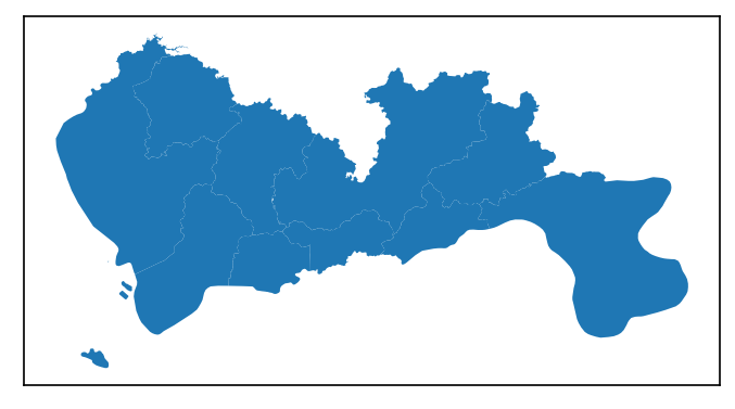
# Read the GeoDataFrame of the study area
sz = gpd.read_file(r'data/sz.json')
sz.crs = None
sz.head()
[2]:
| centroid_x | centroid_y | qh | geometry | |
|---|---|---|---|---|
| 0 | 114.143157 | 22.577605 | 罗湖 | POLYGON ((114.10006 22.53431, 114.10083 22.534... |
| 1 | 114.041535 | 22.546180 | 福田 | POLYGON ((113.98578 22.51348, 114.00553 22.513... |
| 2 | 114.270206 | 22.596432 | 盐田 | POLYGON ((114.19799 22.55673, 114.19817 22.556... |
| 3 | 113.851387 | 22.679120 | 宝安 | MULTIPOLYGON (((113.81831 22.54676, 113.81948 ... |
| 4 | 113.926290 | 22.766157 | 光明 | POLYGON ((113.99768 22.76643, 113.99704 22.766... |
[3]:
fig = plt.figure(1, (8, 3), dpi=150)
ax1 = plt.subplot(111)
sz.plot(ax=ax1)
plt.xticks([], fontsize=10)
plt.yticks([], fontsize=10);
数据预处理
TransBigData集成了几种常见的数据预处理方法。使用“tbd.clean_outofshape”方法,给定研究区域的数据和地理数据帧,可以删除研究区域之外的数据。“tbd.clean_taxi_status”方法可以过滤掉乘客状态瞬时变化的数据(OpenStatus)。使用预处理方法时,需要将相应的列名作为参数传入:
[4]:
# Data Preprocessing
# Delete the data outside of the study area
data = tbd.clean_outofshape(data, sz, col=['Lng', 'Lat'], accuracy=500)

# Delete the data with instantaneous changes in passenger status
data = tbd.clean_taxi_status(data, col=['VehicleNum', 'Time', 'OpenStatus'])
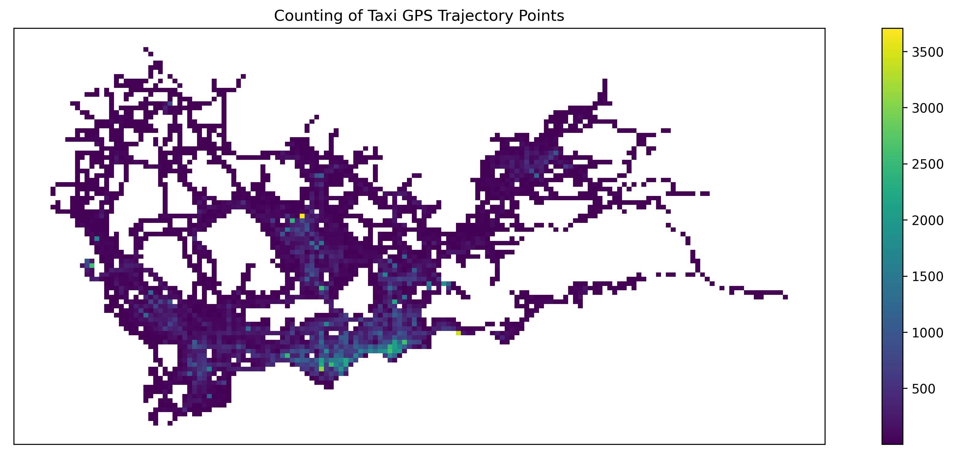
数据网格化
表示数据分布的最基本方法是以地理网格的形式;数据网格化后,每个GPS数据点映射到相应的网格。对于数据网格化,首先需要确定格网参数(可以解释为定义格网坐标系):
[5]:
# Data gridding
# Define the bounds and generate gridding parameters
bounds = [113.6, 22.4, 114.8, 22.9]
params = tbd.area_to_params(bounds, accuracy=500)
print(params)
{'slon': 113.6, 'slat': 22.4, 'deltalon': 0.004872390756896538, 'deltalat': 0.004496605206422906, 'theta': 0, 'method': 'rect', 'gridsize': 500}
获得网格参数后,下一步是将GPS映射到其对应的网格。使用“待定”。GPS_to_grids“,它将生成”LONCOL“列和”LATCOL“列。这两列一起可以指定一个网格:
[6]:
# Mapping GPS data to grids
data['LONCOL'], data['LATCOL'] = tbd.GPS_to_grid(data['Lng'], data['Lat'], params)
data.head()
[6]:
| VehicleNum | Time | Lng | Lat | OpenStatus | Speed | LONCOL | LATCOL | |
|---|---|---|---|---|---|---|---|---|
| 0 | 34745 | 20:27:43 | 113.806847 | 22.623249 | 1 | 27 | 42 | 50 |
| 1 | 27368 | 09:08:53 | 113.805893 | 22.624996 | 0 | 49 | 42 | 50 |
| 2 | 22998 | 10:51:10 | 113.806931 | 22.624166 | 1 | 54 | 42 | 50 |
| 3 | 22998 | 10:11:50 | 113.805946 | 22.625433 | 0 | 43 | 42 | 50 |
| 4 | 22998 | 10:12:05 | 113.806381 | 22.623833 | 0 | 60 | 42 | 50 |
统计每个格子的数据量:
[7]:
# Aggregate data into grids
datatest = data.groupby(['LONCOL', 'LATCOL'])['VehicleNum'].count().reset_index()
datatest.head()
[7]:
| LONCOL | LATCOL | VehicleNum | |
|---|---|---|---|
| 0 | 36 | 63 | 2 |
| 1 | 36 | 66 | 1 |
| 2 | 36 | 67 | 8 |
| 3 | 37 | 62 | 9 |
| 4 | 37 | 63 | 8 |
生成网格的几何图形并将其转换为 GeoDataFrame:
[8]:
# Generate the geometry for grids
datatest['geometry'] = tbd.grid_to_polygon([datatest['LONCOL'], datatest['LATCOL']], params)

# Change it into GeoDataFrame
# import geopandas as gpd
datatest = gpd.GeoDataFrame(datatest)
datatest.head()
[8]:
| LONCOL | LATCOL | VehicleNum | geometry | |
|---|---|---|---|---|
| 0 | 36 | 63 | 2 | POLYGON ((113.77297 22.68104, 113.77784 22.681... |
| 1 | 36 | 66 | 1 | POLYGON ((113.77297 22.69453, 113.77784 22.694... |
| 2 | 36 | 67 | 8 | POLYGON ((113.77297 22.69902, 113.77784 22.699... |
| 3 | 37 | 62 | 9 | POLYGON ((113.77784 22.67654, 113.78271 22.676... |
| 4 | 37 | 63 | 8 | POLYGON ((113.77784 22.68104, 113.78271 22.681... |
绘制生成的网格:
[9]:
# Plot the grids
fig = plt.figure(1, (16, 6), dpi=300)
ax1 = plt.subplot(111)

# tbd.plot_map(plt, bounds, zoom=10, style=4)
datatest.plot(ax=ax1, column='VehicleNum', legend=True)
plt.xticks([], fontsize=10)
plt.yticks([], fontsize=10)
plt.title('Counting of Taxi GPS Trajectory Points', fontsize=12);
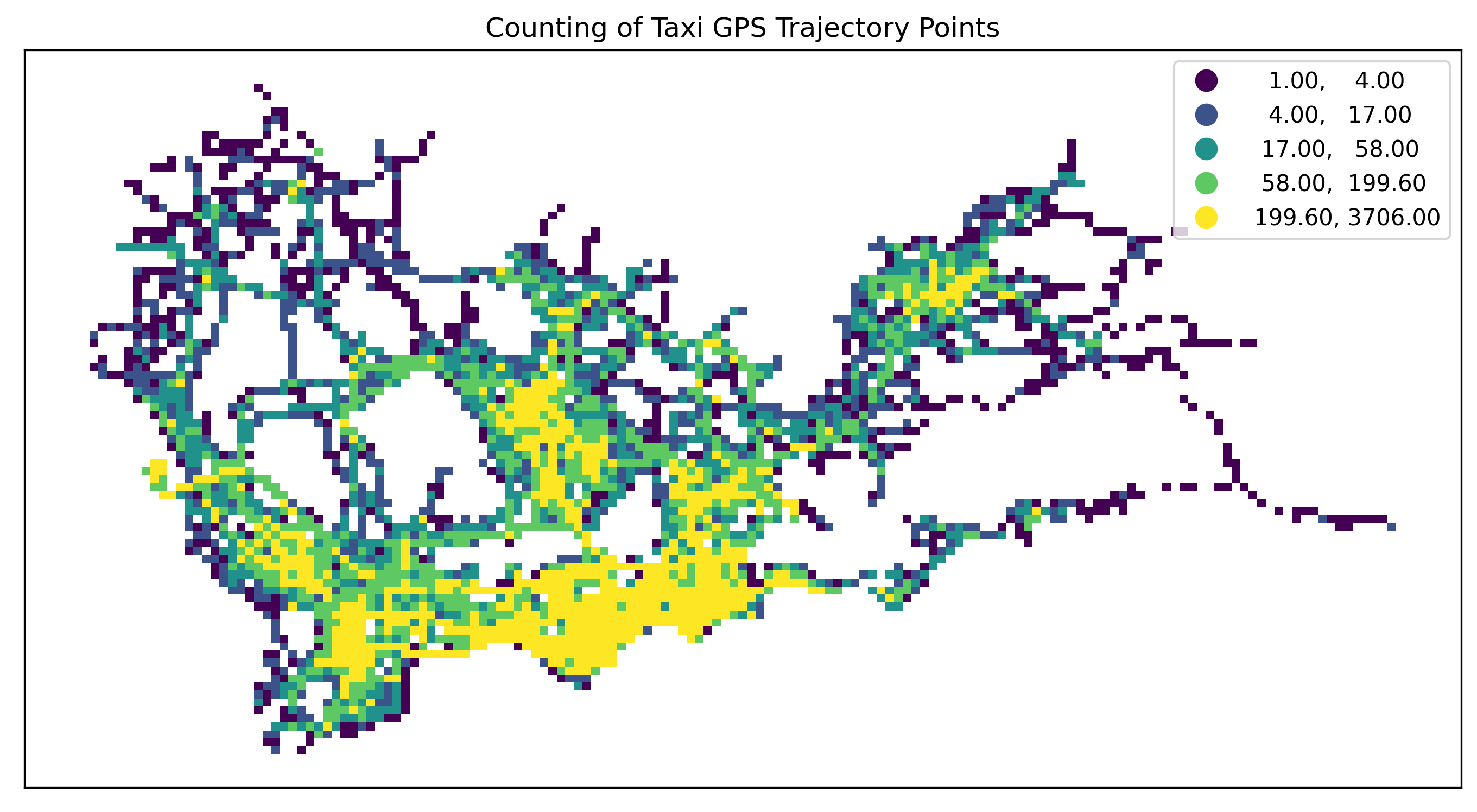
[10]:
# Plot the grids
fig = plt.figure(1, (16, 6), dpi=300) # 确定图形高为6,宽为8;图形清晰度
ax1 = plt.subplot(111)
datatest.plot(ax=ax1, column='VehicleNum', legend=True, scheme='quantiles')
# plt.legend(fontsize=10)
plt.xticks([], fontsize=10)
plt.yticks([], fontsize=10)
plt.title('Counting of Taxi GPS Trajectory Points', fontsize=12);
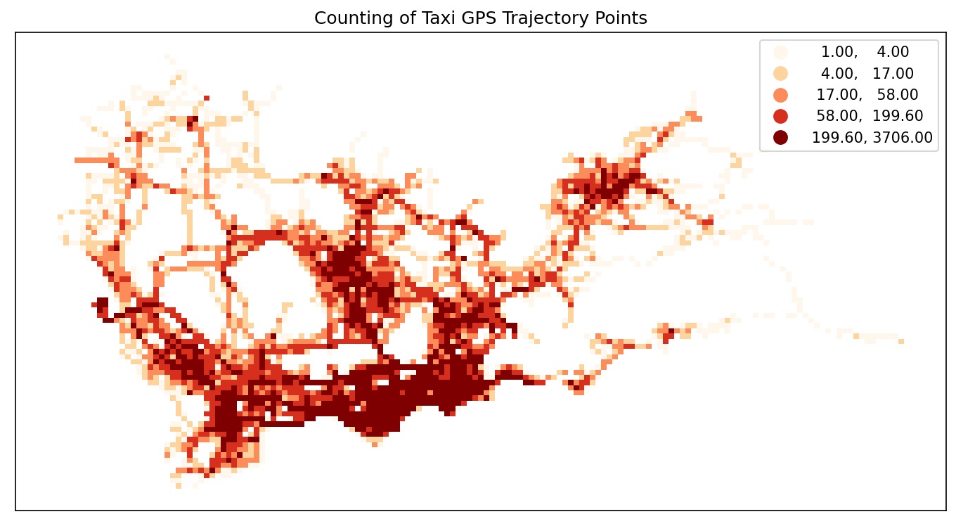
[11]:
# Plot the grids
fig = plt.figure(1, (16, 6), dpi=150) # 确定图形高为6,宽为8;图形清晰度
ax1 = plt.subplot(111)
datatest.plot(ax=ax1, column='VehicleNum', legend=True, cmap='OrRd', scheme='quantiles')
# plt.legend(fontsize=10)
plt.xticks([], fontsize=10)
plt.yticks([], fontsize=10)
plt.title('Counting of Taxi GPS Trajectory Points', fontsize=12);
Origin-destination(OD) 提取和聚合出租车行程
使用“tbd.taxigps_to_od”方法并传入相应的列名以提取出租车行程 OD:
[12]:
# Extract taxi OD from GPS data
oddata = tbd.taxigps_to_od(data,col = ['VehicleNum', 'Time', 'Lng', 'Lat', 'OpenStatus'])
oddata
[12]:
| VehicleNum | stime | slon | slat | etime | elon | elat | ID | |
|---|---|---|---|---|---|---|---|---|
| 427075 | 22396 | 00:19:41 | 114.013016 | 22.664818 | 00:23:01 | 114.021400 | 22.663918 | 0 |
| 131301 | 22396 | 00:41:51 | 114.021767 | 22.640200 | 00:43:44 | 114.026070 | 22.640266 | 1 |
| 417417 | 22396 | 00:45:44 | 114.028099 | 22.645082 | 00:47:44 | 114.030380 | 22.650017 | 2 |
| 376160 | 22396 | 01:08:26 | 114.034897 | 22.616301 | 01:16:34 | 114.035614 | 22.646717 | 3 |
| 21768 | 22396 | 01:26:06 | 114.046021 | 22.641251 | 01:34:48 | 114.066048 | 22.636183 | 4 |
| ... | ... | ... | ... | ... | ... | ... | ... | ... |
| 57666 | 36805 | 22:37:42 | 114.113403 | 22.534767 | 22:48:01 | 114.114365 | 22.550632 | 5332 |
| 175519 | 36805 | 22:49:12 | 114.114365 | 22.550632 | 22:50:40 | 114.115501 | 22.557983 | 5333 |
| 212092 | 36805 | 22:52:07 | 114.115402 | 22.558083 | 23:03:27 | 114.118484 | 22.547867 | 5334 |
| 119041 | 36805 | 23:03:45 | 114.118484 | 22.547867 | 23:20:09 | 114.133286 | 22.617750 | 5335 |
| 224103 | 36805 | 23:36:19 | 114.112968 | 22.549601 | 23:43:12 | 114.089485 | 22.538918 | 5336 |
5337 rows × 8 columns
聚合提取的OD,生成LineString GeoDataFrame
[13]:
# Gridding and aggragate data
od_gdf = tbd.odagg_grid(oddata, params)
od_gdf.head()
/opt/anaconda3/lib/python3.8/site-packages/pandas/core/dtypes/cast.py:91: ShapelyDeprecationWarning: The array interface is deprecated and will no longer work in Shapely 2.0. Convert the '.coords' to a numpy array instead.
  values = construct_1d_object_array_from_listlike(values)
[13]:
| SLONCOL | SLATCOL | ELONCOL | ELATCOL | count | SHBLON | SHBLAT | EHBLON | EHBLAT | geometry | |
|---|---|---|---|---|---|---|---|---|---|---|
| 0 | 40 | 62 | 45 | 68 | 1 | 113.794896 | 22.678790 | 113.819258 | 22.705769 | LINESTRING (113.79490 22.67879, 113.81926 22.7... |
| 3331 | 101 | 36 | 86 | 29 | 1 | 114.092111 | 22.561878 | 114.019026 | 22.530402 | LINESTRING (114.09211 22.56188, 114.01903 22.5... |
| 3330 | 101 | 35 | 105 | 30 | 1 | 114.092111 | 22.557381 | 114.111601 | 22.534898 | LINESTRING (114.09211 22.55738, 114.11160 22.5... |
| 3329 | 101 | 34 | 109 | 34 | 1 | 114.092111 | 22.552885 | 114.131091 | 22.552885 | LINESTRING (114.09211 22.55288, 114.13109 22.5... |
| 3328 | 101 | 34 | 103 | 34 | 1 | 114.092111 | 22.552885 | 114.101856 | 22.552885 | LINESTRING (114.09211 22.55288, 114.10186 22.5... |
[14]:
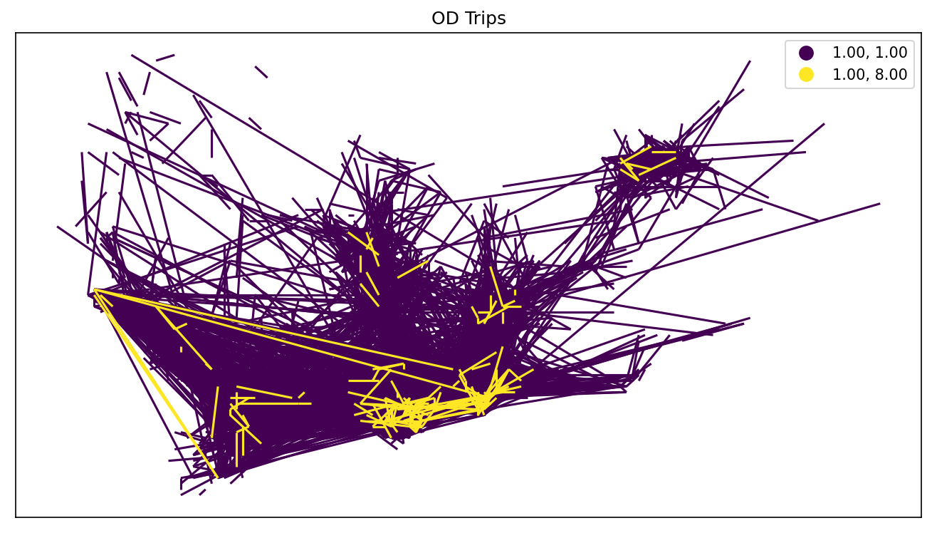
# Plot the grids
fig = plt.figure(1, (16, 6), dpi=150) # 确定图形高为6,宽为8;图形清晰度
ax1 = plt.subplot(111)
# data_grid_count.plot(ax=ax1, column='VehicleNum', legend=True, cmap='OrRd', scheme='quantiles')

od_gdf.plot(ax=ax1, column='count', legend=True, scheme='quantiles')
plt.xticks([], fontsize=10)
plt.yticks([], fontsize=10)
plt.title('OD Trips', fontsize=12);
/opt/anaconda3/lib/python3.8/site-packages/mapclassify/classifiers.py:238: UserWarning: Warning: Not enough unique values in array to form k classes
  Warn(
/opt/anaconda3/lib/python3.8/site-packages/mapclassify/classifiers.py:241: UserWarning: Warning: setting k to 2
  Warn("Warning: setting k to %d" % k_q, UserWarning)
将OD聚合成多边形
``TransBigData``也提供了OD聚合成多边形的方法
[15]:
# Aggragate OD data to polygons
# without passing gridding parameters, the algorithm will map the data
# to polygons directly using their coordinates
od_gdf = tbd.odagg_shape(oddata, sz, round_accuracy=6)
fig = plt.figure(1, (16, 6), dpi=150) # 确定图形高为6,宽为8;图形清晰度
ax1 = plt.subplot(111)
od_gdf.plot(ax=ax1, column='count')
plt.xticks([], fontsize=10)
plt.yticks([], fontsize=10)
plt.title('OD Trips', fontsize=12);
/opt/anaconda3/lib/python3.8/site-packages/pandas/core/dtypes/cast.py:91: ShapelyDeprecationWarning: The array interface is deprecated and will no longer work in Shapely 2.0. Convert the '.coords' to a numpy array instead.
  values = construct_1d_object_array_from_listlike(values)

基于Matplotlib的地图绘制
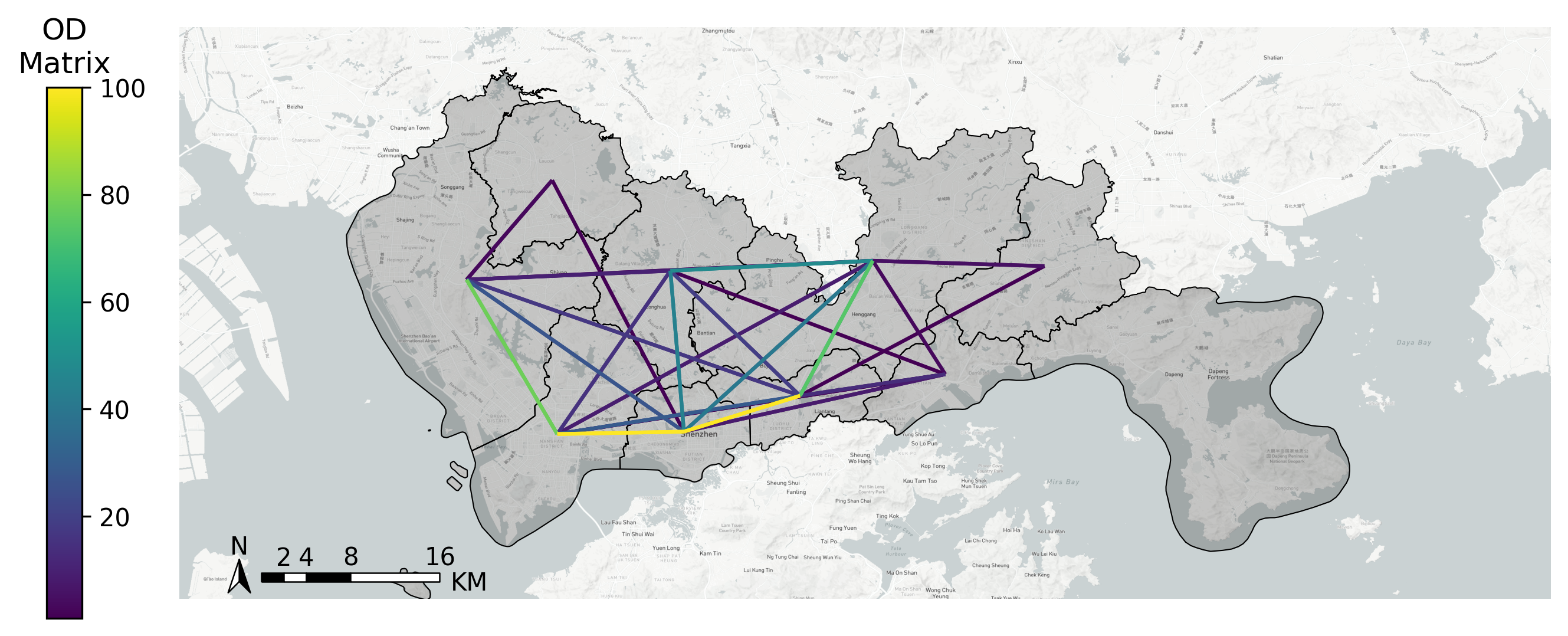
“TransBigData”还在 matplotlib 中提供底图加载。在使用此方法之前,您需要设置底图的mapboxtoken和存储位置,请参阅:“此链接<https://transbigdata.readthedocs.io/en/latest/plot_map.html>”__。“tbd.plot_map”添加底图,tbd.plotscale 添加比例和指南针:
[16]:
# Create figure
fig = plt.figure(1, (10, 10), dpi=300)
ax = plt.subplot(111)
plt.sca(ax)

# Load basemap
tbd.plot_map(plt, bounds, zoom=12, style=4)

# Define an ax for colorbar
cax = plt.axes([0.05, 0.33, 0.02, 0.3])
plt.title('OD\nMatrix')
plt.sca(ax)

# Plot the OD
od_gdf.plot(ax=ax, vmax=100, column='count', cax=cax, legend=True)

# Plot the polygons
sz.plot(ax=ax, edgecolor=(0, 0, 0, 1), facecolor=(0, 0, 0, 0.2), linewidths=0.5)

# Add compass and scale
tbd.plotscale(ax, bounds=bounds, textsize=10, compasssize=1, accuracy=2000, rect=[0.06, 0.03], zorder=10)
plt.axis('off')
plt.xlim(bounds[0], bounds[2])
plt.ylim(bounds[1], bounds[3])
plt.show()
提取出租车轨迹
采用“tbd.taxigps_traj_point”法,输入GPS数据和OD数据,可提取轨迹点
[17]:
data_deliver, data_idle = tbd.taxigps_traj_point(data,oddata,col=['VehicleNum',
                                                                  'Time',
                                                                  'Lng',
                                                                  'Lat',
                                                                  'OpenStatus'])
[18]:
data_deliver.head()
[18]:
| VehicleNum | Time | Lng | Lat | OpenStatus | Speed | LONCOL | LATCOL | ID | flag | |
|---|---|---|---|---|---|---|---|---|---|---|
| 427075 | 22396 | 00:19:41 | 114.013016 | 22.664818 | 1 | 63.0 | 85.0 | 59.0 | 0.0 | 1.0 |
| 427085 | 22396 | 00:19:49 | 114.014030 | 22.665483 | 1 | 55.0 | 85.0 | 59.0 | 0.0 | 1.0 |
| 416622 | 22396 | 00:21:01 | 114.018898 | 22.662500 | 1 | 1.0 | 86.0 | 58.0 | 0.0 | 1.0 |
| 427480 | 22396 | 00:21:41 | 114.019348 | 22.662300 | 1 | 7.0 | 86.0 | 58.0 | 0.0 | 1.0 |
| 416623 | 22396 | 00:22:21 | 114.020615 | 22.663366 | 1 | 0.0 | 86.0 | 59.0 | 0.0 | 1.0 |
[19]:
data_idle.head()
[19]:
| VehicleNum | Time | Lng | Lat | OpenStatus | Speed | LONCOL | LATCOL | ID | flag | |
|---|---|---|---|---|---|---|---|---|---|---|
| 416628 | 22396 | 00:23:01 | 114.021400 | 22.663918 | 0 | 25.0 | 86.0 | 59.0 | 0.0 | 0.0 |
| 401744 | 22396 | 00:25:01 | 114.027115 | 22.662100 | 0 | 25.0 | 88.0 | 58.0 | 0.0 | 0.0 |
| 394630 | 22396 | 00:25:41 | 114.024551 | 22.659834 | 0 | 21.0 | 87.0 | 58.0 | 0.0 | 0.0 |
| 394671 | 22396 | 00:26:21 | 114.022797 | 22.658367 | 0 | 0.0 | 87.0 | 57.0 | 0.0 | 0.0 |
| 394672 | 22396 | 00:26:29 | 114.022797 | 22.658367 | 0 | 0.0 | 87.0 | 57.0 | 0.0 | 0.0 |
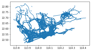
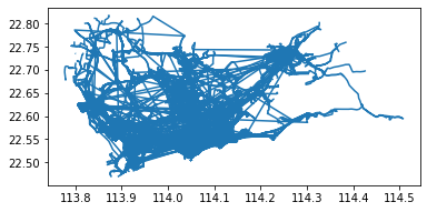
从轨迹点生成投放和空闲轨迹
[20]:
traj_deliver = tbd.points_to_traj(data_deliver)
traj_deliver.plot();
[21]:
traj_idle = tbd.points_to_traj(data_idle[data_idle['OpenStatus'] == 0])
traj_idle.plot()
[21]:
<AxesSubplot:>
轨迹可视化
“TransBigData”的内置可视化功能利用可视化包“keplergl”,使用简单的代码以交互方式可视化Jupyter笔记本上的数据。要使用此方法,请为 python 安装 ‘’keplergl’ 包:
pip 安装 keplergl
详细信息请参阅“此链接<https://transbigdata.readthedocs.io/en/latest/visualization.html>”__
轨迹数据可视化:
[22]:
tbd.visualization_trip(data_deliver)
Processing trajectory data...
Generate visualization...
User Guide: https://docs.kepler.gl/docs/keplergl-jupyter