数据栅格化

`area_to_grid`(location[, accuracy, method, ...])	在边界或形状中生成矩形栅格
`area_to_params`(location[, accuracy, method])	生成栅格化参数
`GPS_to_grid`(lon, lat, params)	将 GPS 数据与栅格匹配。
`grid_to_centre`(gridid, params)	栅格的中心位置。
`grid_to_polygon`(gridid, params)	根据栅格ID生成几何列。
`grid_to_area`(data, shape, params[, col])	输入格网 ID 两列、地理面和格网参数。
`grid_to_params`(grid)	从栅格重新生成栅格化参数。
`grid_params_optimize`(data, initialparams[, ...])	优化栅格参数
`geohash_encode`(lon, lat[, precision])	输入经纬度和精度，编码geohash码
`geohash_decode`(geohash)	解码geohash码
`geohash_togrid`(geohash)	输入geohash码生成geohash栅格单元格

栅格化框架

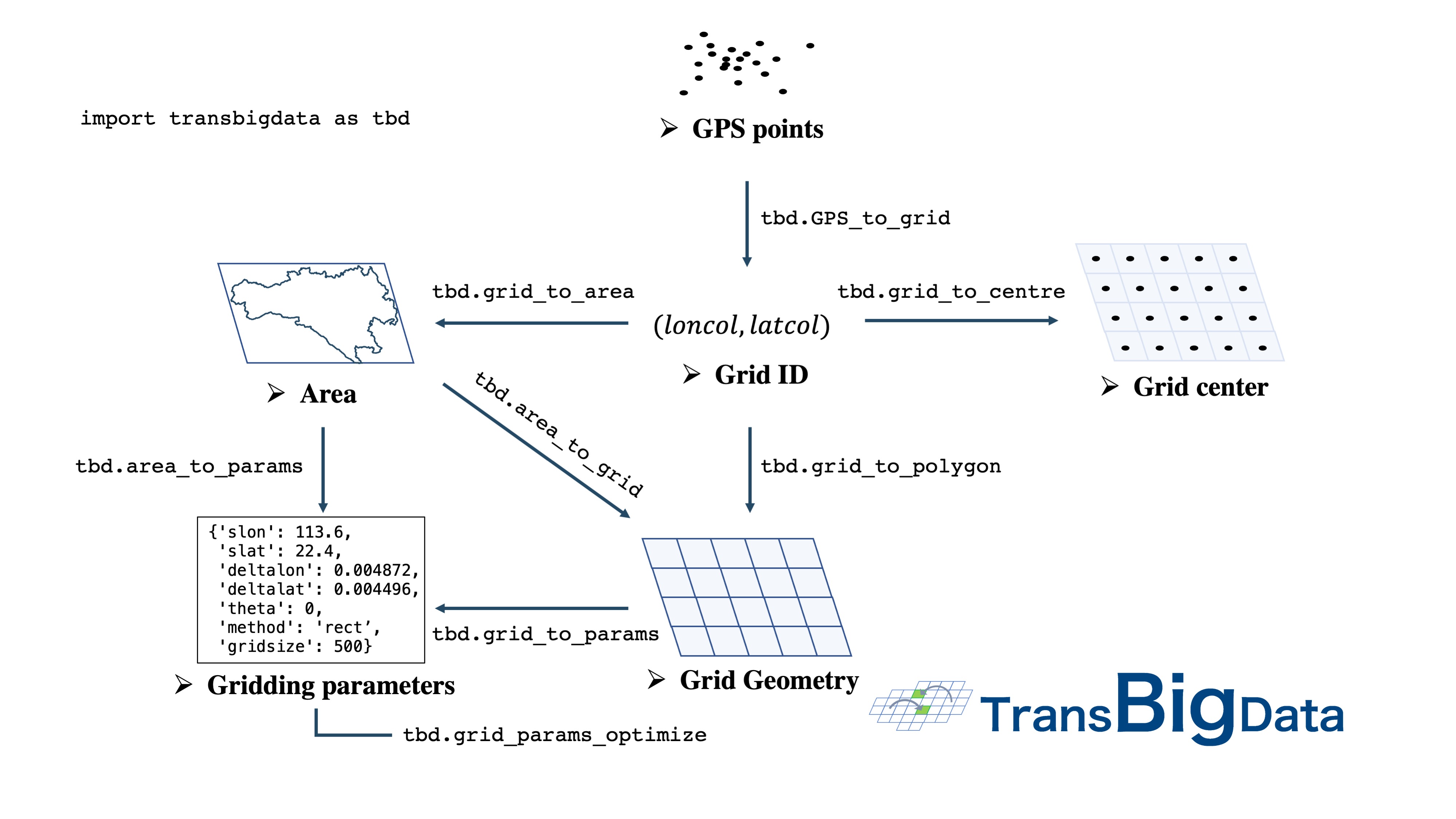
transbigdata.area_to_grid(location, accuracy=500, method='rect', params='auto')

在边界或形状中生成矩形栅格

参数:

location (bounds(List) or shape(GeoDataFrame)) – 生成栅格的位置。如果边界为 [lon1， lat1， lon2， lat2]（WGS84），其中 lon1 ， lat1 是左下角坐标，lon2 ， lat2 是右上角坐标如果是形状，则应为 GeoDataFrame
accuracy (number) – 栅格尺寸（米）
method (str) – 直角、三角或六角
params (list or dict) – 栅格化参数。有关栅格化参数的详细信息，请参阅 https://transbigdata.readthedocs.io/en/latest/grids.html。给出格网参数时，将不使用精度。

返回:

grid （GeoDataFrame） – Grid GeoDataFrame、LONCOL 和 LATCOL 是栅格的索引，HBLON 和 HBLAT 是栅格的中心
参数（列表或字典） – 栅格参数。有关栅格化参数的详细信息，请参阅 https://transbigdata.readthedocs.io/en/latest/grids.html。

transbigdata.area_to_params(location, accuracy=500, method='rect')

生成栅格化参数

参数:

location (bounds(List) or shape(GeoDataFrame)) – 生成栅格的位置。如果边界为 [lon1， lat1， lon2， lat2]（WGS84），其中 lon1 ， lat1 是左下角坐标，lon2 ， lat2 是右上角坐标如果是形状，则应为 GeoDataFrame
accuracy (number) – 栅格尺寸（米）
method (str) – 直角、三角或六角

返回:

参数 – 栅格参数。有关栅格化参数的详细信息，请参阅 https://transbigdata.readthedocs.io/en/latest/grids.html。

返回类型:

list or dict

transbigdata.GPS_to_grid(lon, lat, params)

将 GPS 数据与栅格匹配。输入是经度、纬度和格网参数列。输出是栅格 ID。

参数:

lon (Series) – 经度栏
lat (Series) – 纬度栏
params (list or dict) – 栅格化参数。有关栅格化参数的详细信息，请参阅 https://transbigdata.readthedocs.io/en/latest/grids.html。

返回:

矩形栅格
[LONCOL，LATCOL] （list） – 两列 LONCOL 和 LATCOL 一起可以指定栅格。
三角形和六边形栅格
[loncol_1，loncol_2，loncol_3] （list） – 栅格纬度的索引。两列 LONCOL 和 LATCOL 一起可以指定一个栅格。

transbigdata.grid_to_centre(gridid, params)

栅格的中心位置。输入是格网ID和参数，输出是格网中心位置。

参数:

gridid (list) – 如果“矩形栅格”[LONCOL，LATCOL]：系列两列 LONCOL 和 LATCOL 一起可以指定栅格。如果“三角形和六边形栅格” [loncol_1，loncol_2，loncol_3] ：系列栅格纬度的索引。两列 LONCOL 和 LATCOL 一起可以指定一个栅格。
params (list or dict) – 栅格化参数。有关栅格化参数的详细信息，请参阅 https://transbigdata.readthedocs.io/en/latest/grids.html。

返回:

HBLON (Series) – 栅格中心的经度
HBLAT (Series) – 栅格中心的纬度

transbigdata.grid_to_polygon(gridid, params)

基于格网 ID 生成几何列。输入是栅格 ID，输出是几何图形。支持矩形、三角形和六边形栅格

参数:

gridid (list) – 如果“矩形栅格”[LONCOL，LATCOL]：系列两列 LONCOL 和 LATCOL 一起可以指定栅格。如果“三角形和六边形栅格” [loncol_1，loncol_2，loncol_3] ：系列栅格纬度的索引。两列 LONCOL 和 LATCOL 一起可以指定一个栅格。
params (list or dict) – 栅格化参数。有关栅格化参数的详细信息，请参阅 https://transbigdata.readthedocs.io/en/latest/grids.html。

返回:

geometry – 栅格地理多边形的列

返回类型:

Series

transbigdata.grid_to_area(data, shape, params, col=['LONCOL', 'LATCOL'])

输入格网 ID 两列、地理面和格网参数。输出是栅格。

参数:

data (DataFrame) – 数据，有两列栅格ID
shape (GeoDataFrame) – 地理多边形
params (list or dict) – 栅格化参数。有关栅格化参数的详细信息，请参阅 https://transbigdata.readthedocs.io/en/latest/grids.html。
col (List) – 列名称 [LONCOL，LATCOL] 用于矩形栅格，或 [loncol_1，loncol_2，loncol_3] 表示三和六栅格

返回:

data1 – 数据栅格化和映射到相应的地理多边形

返回类型:

DataFrame

transbigdata.grid_to_params(grid)

从栅格重新生成栅格化参数。

参数:: grid (GeoDataFrame) – transbigdata生成的栅格
返回:: 参数 – 栅格参数。有关栅格化参数的详细信息，请参阅 https://transbigdata.readthedocs.io/en/latest/grids.html。
返回类型:: list or dict

transbigdata.grid_params_optimize(data, initialparams, col=['uid', 'lon', 'lat'], optmethod='centerdist', printlog=False, sample=0, pop=15, max_iter=50, w=0.1, c1=0.5, c2=0.5)

优化栅格参数

参数:

data (DataFrame) – 轨迹数据
initialparams (List) – 初始栅格参数
col (List) – 列名[uid,lon,lat]
optmethod (str) – 优化方法：centerdist, gini, gridscount
printlog (bool) – 是否打印明细结果
sample (int) – 采样数据作为输入，为0则不采样
pop – 来自 scikit-opt 的 PSO 中的参数
max_iter – 来自 scikit-opt 的 PSO 中的参数
w – 来自 scikit-opt 的 PSO 中的参数
c1 – 来自 scikit-opt 的 PSO 中的参数
c2 – 来自 scikit-opt 的 PSO 中的参数

返回:

params_optimized – 优化的参数

返回类型:

List

geohash编码

Geohash 是一种公共地理编码系统，可将纬度和经度地理位置编码为字母和数字字符串，这些字符串也可以解码回纬度和经度。每个字符串代表一个栅格编号，字符串的长度越长，精度越高。根据wiki<https://en.wikipedia.org/wiki/Geohash>，与精度对应的Geohash字符串长度表如下。

geohash 长度（精度）	纬度位	lng位	纬度错误	lng 错误	公里错误
1	2	3	±23	±23	±2500
2	5	5	±2.8	±5.6	±630
3	7	8	±0.70	±0.70	±78
4	10	10	±0.087	±0.18	±20
5	12	13	±0.022	±0.022	±2.4
6	15	15	±0.0027	±0.0055	±0.61
7	17	18	±0.00068	±0.00068	±0.076
8	20	20	±0.000085	±0.00017	±0.019

TransBigData还提供了基于Geohash的功能，三个功能如下：

transbigdata.geohash_encode(lon, lat, precision=12)

输入经纬度和精度，编码geohash码

参数:

lon (Series) – 经度系列
lat (Series) – 纬度系列
precision (number) – geohash精度

返回:

geohash – 编码的geohash系列

返回类型:

Series

transbigdata.geohash_decode(geohash)

解码geohash码

参数:

geohash (Series) – encoded geohash 系列

返回:

lon (Series) – 解码后的经度系列
lat (Series) – 解码后的纬度系列

transbigdata.geohash_togrid(geohash)

输入geohash码生成geohash栅格单元格

参数:: geohash (Series) – encoded geohash 系列
返回:: poly – geohash 的栅格单元多边形
返回类型:: Series

与TransBigData软件包中提供的矩形网格处理方法相比，geohash速度较慢，并且不提供自由定义的网格大小。以下示例演示如何使用这三个函数来利用 geohash 编码、解码和可视化

import transbigdata as tbd
import pandas as pd
import geopandas as gpd
#read data
data = pd.read_csv('TaxiData-Sample.csv',header = None)
data.columns = ['VehicleNum','time','slon','slat','OpenStatus','Speed']

#encode geohash
data['geohash'] = tbd.geohash_encode(data['slon'],data['slat'],precision=6)
data['geohash']

0         ws0btw
1         ws0btz
2         ws0btz
3         ws0btz
4         ws0by4
           ...
544994    ws131q
544995    ws1313
544996    ws131f
544997    ws1361
544998    ws10tq
Name: geohash, Length: 544999, dtype: object

#Aggregate
dataagg = data.groupby(['geohash'])['VehicleNum'].count().reset_index()
dataagg['lon_geohash'],dataagg['lat_geohash'] = tbd.geohash_decode(dataagg['geohash'])
dataagg['geometry'] = tbd.geohash_togrid(dataagg['geohash'])
dataagg = gpd.GeoDataFrame(dataagg)
dataagg

	geohash	VehicleNum	lon_geohash	lat_geohash	geometry
0	w3uf3x	1	108.	10.28	POLYGON ((107.99561 10.27771, 107.99561 10.283...
1	webzz6	12	113.9	22.47	POLYGON ((113.87329 22.46704, 113.87329 22.472...
2	webzz7	21	113.9	22.48	POLYGON ((113.87329 22.47253, 113.87329 22.478...
3	webzzd	1	113.9	22.47	POLYGON ((113.88428 22.46704, 113.88428 22.472...
4	webzzf	2	113.9	22.47	POLYGON ((113.89526 22.46704, 113.89526 22.472...
...	...	...	...	...	...
2022	ws1d9u	1	114.7	22.96	POLYGON ((114.68628 22.96143, 114.68628 22.966...
2023	ws1ddh	6	114.7	22.96	POLYGON ((114.69727 22.96143, 114.69727 22.966...
2024	ws1ddj	2	114.7	22.97	POLYGON ((114.69727 22.96692, 114.69727 22.972...
2025	ws1ddm	4	114.7	22.97	POLYGON ((114.70825 22.96692, 114.70825 22.972...
2026	ws1ddq	7	114.7	22.98	POLYGON ((114.70825 22.97241, 114.70825 22.977...

2027 rows × 5 columns

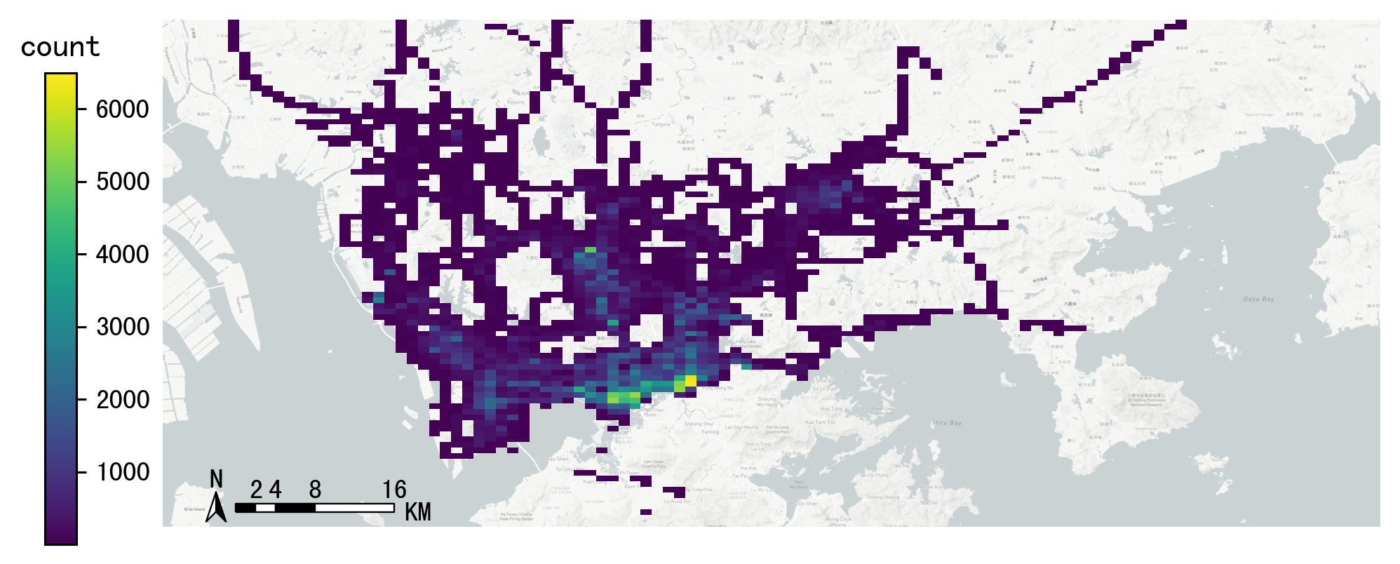
bounds = [113.6,22.4,114.8,22.9]
import matplotlib.pyplot as plt
import plot_map
fig =plt.figure(1,(8,8),dpi=280)
ax =plt.subplot(111)
plt.sca(ax)
tbd.plot_map(plt,bounds,zoom = 12,style = 4)
cax = plt.axes([0.05, 0.33, 0.02, 0.3])
plt.title('count')
plt.sca(ax)
dataagg.plot(ax = ax,column = 'VehicleNum',cax = cax,legend = True)
tbd.plotscale(ax,bounds = bounds,textsize = 10,compasssize = 1,accuracy = 2000,rect = [0.06,0.03],zorder = 10)
plt.axis('off')
plt.xlim(bounds[0],bounds[2])
plt.ylim(bounds[1],bounds[3])
plt.show()