8 Community detection for bicycle-sharing demand
For bicycle sharing demand, each trip of can be seen as a process from the starting loaction to the end loaction. When we regard the start point and the end point as nodes, and the travel between them as edges, a network can be constructed. By analysing this network, we can get information about the spatial connection structure of the city or the macro travel characteristics of the bicycle sharing demand.
Community detection, also called graph partition, helps us to reveal the hidden relations among the nodes in the network. In this example, we will introduce how to integrate TransBigData into the analysis process of community detection from bicycle-sharing data.
To run this example, you may have to install igraph and seaborn:
pip install igraphpip install seaborn
Data preprocessing
[1]:
# Fristly, import packages.
import pandas as pd
import numpy as np
import geopandas as gpd
import transbigdata as tbd
[2]:
#Read bicycle sharing data
bikedata = pd.read_csv(r'data/bikedata-sample.csv')
bikedata.head(5)
[2]:
| BIKE_ID | DATA_TIME | LOCK_STATUS | LONGITUDE | LATITUDE | |
|---|---|---|---|---|---|
| 0 | 5 | 2018-09-01 0:00:36 | 1 | 121.363566 | 31.259615 |
| 1 | 6 | 2018-09-01 0:00:50 | 0 | 121.406226 | 31.214436 |
| 2 | 6 | 2018-09-01 0:03:01 | 1 | 121.409402 | 31.215259 |
| 3 | 6 | 2018-09-01 0:24:53 | 0 | 121.409228 | 31.214427 |
| 4 | 6 | 2018-09-01 0:26:38 | 1 | 121.409771 | 31.214406 |
[3]:
#Read the polygon of the study area
shanghai_admin = gpd.read_file(r'data/shanghai.json')
#delete the data outside of the study area
bikedata = tbd.clean_outofshape(bikedata, shanghai_admin, col=['LONGITUDE', 'LATITUDE'], accuracy=500)
Identify Bicycle sharing trip information using tbd.bikedata_to_od
[4]:
move_data,stop_data = tbd.bikedata_to_od(bikedata,
                   col = ['BIKE_ID','DATA_TIME','LONGITUDE','LATITUDE','LOCK_STATUS'])
move_data.head(5)
[4]:
| BIKE_ID | stime | slon | slat | etime | elon | elat | |
|---|---|---|---|---|---|---|---|
| 96 | 6 | 2018-09-01 0:00:50 | 121.406226 | 31.214436 | 2018-09-01 0:03:01 | 121.409402 | 31.215259 |
| 561 | 6 | 2018-09-01 0:24:53 | 121.409228 | 31.214427 | 2018-09-01 0:26:38 | 121.409771 | 31.214406 |
| 564 | 6 | 2018-09-01 0:50:16 | 121.409727 | 31.214403 | 2018-09-01 0:52:14 | 121.412610 | 31.214905 |
| 784 | 6 | 2018-09-01 0:53:38 | 121.413333 | 31.214951 | 2018-09-01 0:55:38 | 121.412656 | 31.217051 |
| 1028 | 6 | 2018-09-01 11:35:01 | 121.419261 | 31.213414 | 2018-09-01 11:35:13 | 121.419518 | 31.213657 |
[5]:
#Calculate the travel distance
move_data['distance'] = tbd.getdistance(move_data['slon'],move_data['slat'],move_data['elon'],move_data['elat'])
#Remove too long and too short trips
move_data = move_data[(move_data['distance']>100)&(move_data['distance']<10000)]
Perform data gridding:
[6]:
#obtain gridding params
bounds = (120.85, 30.67, 122.24, 31.87)
params = tbd.grid_params(bounds,accuracy = 500)
#aggregate the travel informations
od_gdf = tbd.odagg_grid(move_data, params, col=['slon', 'slat', 'elon', 'elat'])
od_gdf.head(5)
/opt/anaconda3/envs/transbigdata/lib/python3.9/site-packages/pandas/core/dtypes/cast.py:122: ShapelyDeprecationWarning: The array interface is deprecated and will no longer work in Shapely 2.0. Convert the '.coords' to a numpy array instead.
  arr = construct_1d_object_array_from_listlike(values)
[6]:
| SLONCOL | SLATCOL | ELONCOL | ELATCOL | count | SHBLON | SHBLAT | EHBLON | EHBLAT | geometry | |
|---|---|---|---|---|---|---|---|---|---|---|
| 0 | 26 | 95 | 26 | 96 | 1 | 120.986782 | 31.097177 | 120.986782 | 31.101674 | LINESTRING (120.98678 31.09718, 120.98678 31.1... |
| 40803 | 117 | 129 | 116 | 127 | 1 | 121.465519 | 31.250062 | 121.460258 | 31.241069 | LINESTRING (121.46552 31.25006, 121.46026 31.2... |
| 40807 | 117 | 129 | 117 | 128 | 1 | 121.465519 | 31.250062 | 121.465519 | 31.245565 | LINESTRING (121.46552 31.25006, 121.46552 31.2... |
| 40810 | 117 | 129 | 117 | 131 | 1 | 121.465519 | 31.250062 | 121.465519 | 31.259055 | LINESTRING (121.46552 31.25006, 121.46552 31.2... |
| 40811 | 117 | 129 | 118 | 126 | 1 | 121.465519 | 31.250062 | 121.470780 | 31.236572 | LINESTRING (121.46552 31.25006, 121.47078 31.2... |
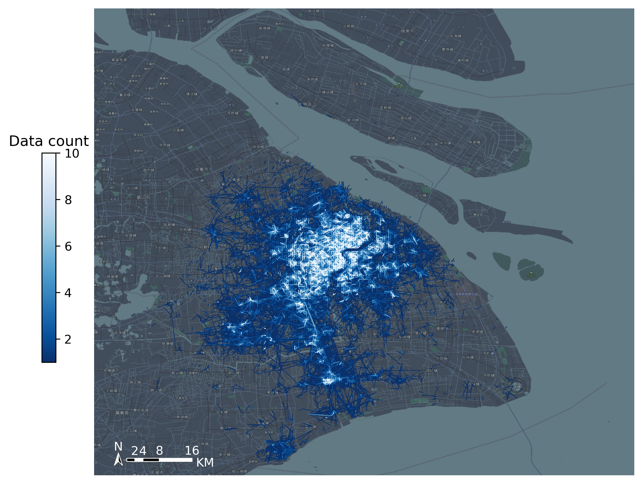
Visualize the OD data
[7]:
#Create figure
import matplotlib.pyplot as plt
fig =plt.figure(1,(8,8),dpi=300)
ax =plt.subplot(111)
plt.sca(ax)

#Load basemap
tbd.plot_map(plt,bounds,zoom = 11,style = 8)

#Create colorbar
cax = plt.axes([0.05, 0.33, 0.02, 0.3])
plt.title('Data count')
plt.sca(ax)

#Plot OD
od_gdf.plot(ax = ax,column = 'count',cmap = 'Blues_r',linewidth = 0.5,vmax = 10,cax = cax,legend = True)

#Plot compass and scale
tbd.plotscale(ax,bounds = bounds,textsize = 10,compasssize = 1,textcolor = 'white',accuracy = 2000,rect = [0.06,0.03],zorder = 10)
plt.axis('off')
plt.xlim(bounds[0],bounds[2])
plt.ylim(bounds[1],bounds[3])
plt.show()
Create Network
Extract node data
Combine the LONCOL and LATCOL columns into one field and extract node set
[8]:
#Combine the ``LONCOL`` and ``LATCOL`` columns into one field
od_gdf['S'] = od_gdf['SLONCOL'].astype(str) + ',' + od_gdf['SLATCOL'].astype(str)
od_gdf['E'] = od_gdf['ELONCOL'].astype(str) + ',' + od_gdf['ELATCOL'].astype(str)
#extract node set
node = set(od_gdf['S'])|set(od_gdf['E'])
node = pd.DataFrame(node)
#reindex the node
node['id'] = range(len(node))
node
[8]:
| 0 | id | |
|---|---|---|
| 0 | 164,81 | 0 |
| 1 | 71,125 | 1 |
| 2 | 102,118 | 2 |
| 3 | 125,115 | 3 |
| 4 | 143,76 | 4 |
| ... | ... | ... |
| 9806 | 98,167 | 9806 |
| 9807 | 46,130 | 9807 |
| 9808 | 118,82 | 9808 |
| 9809 | 158,57 | 9809 |
| 9810 | 104,169 | 9810 |
9811 rows × 2 columns
Extract edge data
[9]:
#Merge the node information to the OD data to extract edge data.
node.columns = ['S','S_id']
od_gdf = pd.merge(od_gdf,node,on = ['S'])
node.columns = ['E','E_id']
od_gdf = pd.merge(od_gdf,node,on = ['E'])
#Extract edge data
edge = od_gdf[['S_id','E_id','count']]
edge
[9]:
| S_id | E_id | count | |
|---|---|---|---|
| 0 | 6251 | 4211 | 1 |
| 1 | 5879 | 8676 | 1 |
| 2 | 8432 | 8676 | 3 |
| 3 | 5511 | 8676 | 1 |
| 4 | 3386 | 8676 | 1 |
| ... | ... | ... | ... |
| 68468 | 5663 | 5835 | 2 |
| 68469 | 7738 | 4266 | 2 |
| 68470 | 360 | 8003 | 2 |
| 68471 | 6759 | 601 | 3 |
| 68472 | 6081 | 3107 | 3 |
68473 rows × 3 columns
Create Network
[10]:
import igraph
#Create Network
g = igraph.Graph()
#Add node
g.add_vertices(len(node))
#Add edge
g.add_edges(edge[['S_id','E_id']].values)
#Add weight
edge_weights = edge[['count']].values
for i in range(len(edge_weights)):
    g.es[i]['weight'] = edge_weights[i]
Community detection
[11]:
#Community detection
g_clustered = g.community_multilevel(weights = edge_weights, return_levels=False)
[12]:
#Modularity
g_clustered.modularity
[12]:
0.8496074605497185
[13]:
#Assign the group result to the node
node['group'] = g_clustered.membership
#rename the columns
node.columns = ['grid','node_id','group']
node
[13]:
| grid | node_id | group | |
|---|---|---|---|
| 0 | 164,81 | 0 | 0 |
| 1 | 71,125 | 1 | 1 |
| 2 | 102,118 | 2 | 2 |
| 3 | 125,115 | 3 | 3 |
| 4 | 143,76 | 4 | 4 |
| ... | ... | ... | ... |
| 9806 | 98,167 | 9806 | 9 |
| 9807 | 46,130 | 9807 | 555 |
| 9808 | 118,82 | 9808 | 6 |
| 9809 | 158,57 | 9809 | 132 |
| 9810 | 104,169 | 9810 | 86 |
9811 rows × 3 columns
Visualize the community
[14]:
#Count the number of grids per community
group = node['group'].value_counts()
#Extract communities with more than 10 grids
group = group[group>10]
#Retain only these community grids
node = node[node['group'].apply(lambda r:r in group.index)]

#Get the grid number
node['LONCOL'] = node['grid'].apply(lambda r:r.split(',')[0]).astype(int)
node['LATCOL'] = node['grid'].apply(lambda r:r.split(',')[1]).astype(int)
#Generate the geometry
node['geometry'] = tbd.gridid_to_polygon(node['LONCOL'],node['LATCOL'],params)
#Change it into GeoDataFrame
import geopandas as gpd
node = gpd.GeoDataFrame(node)
node
/var/folders/b0/q8rx9fj965b5p7yqq8zhvdx80000gn/T/ipykernel_30130/418053260.py:9: SettingWithCopyWarning:
A value is trying to be set on a copy of a slice from a DataFrame.
Try using .loc[row_indexer,col_indexer] = value instead

See the caveats in the documentation: https://pandas.pydata.org/pandas-docs/stable/user_guide/indexing.html#returning-a-view-versus-a-copy
  node['LONCOL'] = node['grid'].apply(lambda r:r.split(',')[0]).astype(int)
/var/folders/b0/q8rx9fj965b5p7yqq8zhvdx80000gn/T/ipykernel_30130/418053260.py:10: SettingWithCopyWarning:
A value is trying to be set on a copy of a slice from a DataFrame.
Try using .loc[row_indexer,col_indexer] = value instead

See the caveats in the documentation: https://pandas.pydata.org/pandas-docs/stable/user_guide/indexing.html#returning-a-view-versus-a-copy
  node['LATCOL'] = node['grid'].apply(lambda r:r.split(',')[1]).astype(int)
/var/folders/b0/q8rx9fj965b5p7yqq8zhvdx80000gn/T/ipykernel_30130/418053260.py:12: SettingWithCopyWarning:
A value is trying to be set on a copy of a slice from a DataFrame.
Try using .loc[row_indexer,col_indexer] = value instead

See the caveats in the documentation: https://pandas.pydata.org/pandas-docs/stable/user_guide/indexing.html#returning-a-view-versus-a-copy
  node['geometry'] = tbd.gridid_to_polygon(node['LONCOL'],node['LATCOL'],params)
[14]:
| grid | node_id | group | LONCOL | LATCOL | geometry | |
|---|---|---|---|---|---|---|
| 1 | 71,125 | 1 | 1 | 71 | 125 | POLYGON ((121.22089 31.22983, 121.22615 31.229... |
| 2 | 102,118 | 2 | 2 | 102 | 118 | POLYGON ((121.38398 31.19835, 121.38924 31.198... |
| 3 | 125,115 | 3 | 3 | 125 | 115 | POLYGON ((121.50498 31.18486, 121.51024 31.184... |
| 4 | 143,76 | 4 | 4 | 143 | 76 | POLYGON ((121.59967 31.00949, 121.60493 31.009... |
| 5 | 142,87 | 5 | 4 | 142 | 87 | POLYGON ((121.59441 31.05896, 121.59967 31.058... |
| ... | ... | ... | ... | ... | ... | ... |
| 9802 | 103,103 | 9802 | 8 | 103 | 103 | POLYGON ((121.38924 31.13090, 121.39450 31.130... |
| 9803 | 162,133 | 9803 | 28 | 162 | 133 | POLYGON ((121.69963 31.26580, 121.70489 31.265... |
| 9804 | 107,130 | 9804 | 41 | 107 | 130 | POLYGON ((121.41028 31.25231, 121.41554 31.252... |
| 9806 | 98,167 | 9806 | 9 | 98 | 167 | POLYGON ((121.36293 31.41868, 121.36819 31.418... |
| 9808 | 118,82 | 9808 | 6 | 118 | 82 | POLYGON ((121.46815 31.03647, 121.47341 31.036... |
8522 rows × 6 columns
[15]:
node.plot('group')
[15]:
<AxesSubplot:>

[16]:
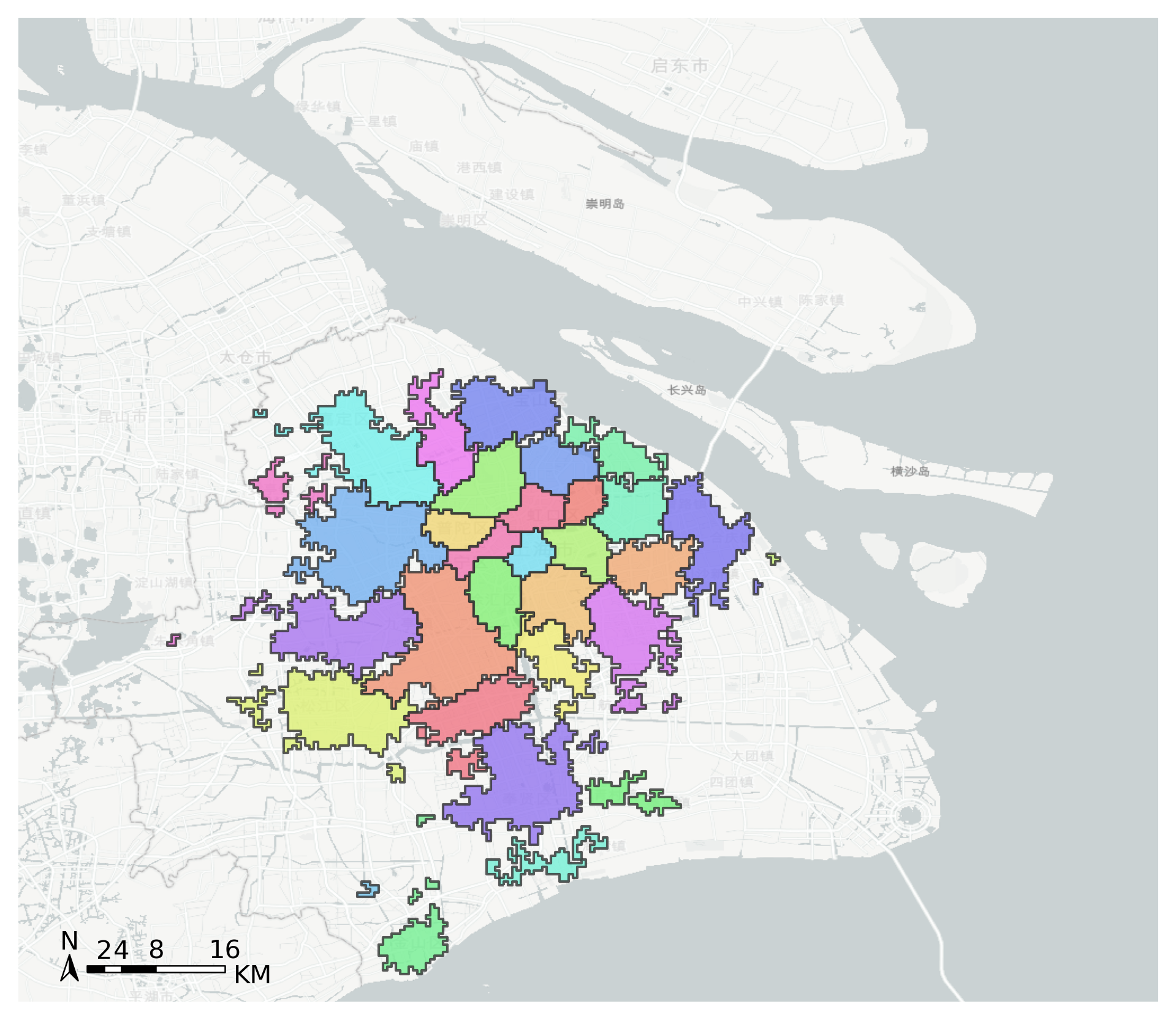
#Use the group column to merge polygon
node_community = tbd.merge_polygon(node,'group')
#Input polygon GeoDataFrame data, take the exterior boundary of the polygon to form a new polygon
node_community = tbd.polyon_exterior(node_community,minarea = 0.000100)
/opt/anaconda3/envs/transbigdata/lib/python3.9/site-packages/transbigdata/gisprocess.py:205: ShapelyDeprecationWarning: Iteration over multi-part geometries is deprecated and will be removed in Shapely 2.0. Use the `geoms` property to access the constituent parts of a multi-part geometry.
  for i in p:
[17]:
#Generate palette
import seaborn as sns
## l: Luminance
## s: Saturation
cmap = sns.hls_palette(n_colors=len(node_community), l=.7, s=0.8)
sns.palplot(cmap)

[19]:
#Create figure
import matplotlib.pyplot as plt
fig =plt.figure(1,(8,8),dpi=300)
ax =plt.subplot(111)
plt.sca(ax)
#Load basemap
tbd.plot_map(plt,bounds,zoom = 10,style = 6)
#Set colormap
from matplotlib.colors import ListedColormap
#Disrupting the order of the community
node_community = node_community.sample(frac=1)
#Plot community
node_community.plot(cmap = ListedColormap(cmap),ax = ax,edgecolor = '#333',alpha = 0.8)
#Add scale
tbd.plotscale(ax,bounds = bounds,textsize = 10,compasssize = 1,textcolor = 'k'
              ,accuracy = 2000,rect = [0.06,0.03],zorder = 10)
plt.axis('off')
plt.xlim(bounds[0],bounds[2])
plt.ylim(bounds[1],bounds[3])
plt.show()