8 共享单车出行需求的社区发现
对于共享单车需求来说,每一次出行都可以看作是从起点到终点的一段过程。当我们把起点和终点看成节点,把它们之间的行程当作边时,就可以构建一个网络。通过分析该网络,我们可以得到有关城市空间连接结构或共享单车需求的宏观出行特征的信息。
社区检测,也称为图分区,帮助我们揭示网络中节点之间的隐藏关系。在这个例子中,我们将介绍如何从共享单车数据将TransBigData集成到社区检测的分析过程中。
要运行这个例子,你可能必须安装``igraph``和``seaborn``:
pip install igraphpip install seaborn
数据预处理
[1]:
# Fristly, import packages.
import pandas as pd
import numpy as np
import geopandas as gpd
import transbigdata as tbd
[2]:
#Read bicycle sharing data
bikedata = pd.read_csv(r'data/bikedata-sample.csv')
bikedata.head(5)
[2]:
| BIKE_ID | DATA_TIME | LOCK_STATUS | LONGITUDE | LATITUDE | |
|---|---|---|---|---|---|
| 0 | 5 | 2018-09-01 0:00:36 | 1 | 121.363566 | 31.259615 |
| 1 | 6 | 2018-09-01 0:00:50 | 0 | 121.406226 | 31.214436 |
| 2 | 6 | 2018-09-01 0:03:01 | 1 | 121.409402 | 31.215259 |
| 3 | 6 | 2018-09-01 0:24:53 | 0 | 121.409228 | 31.214427 |
| 4 | 6 | 2018-09-01 0:26:38 | 1 | 121.409771 | 31.214406 |
[3]:
#Read the polygon of the study area
shanghai_admin = gpd.read_file(r'data/shanghai.json')
#delete the data outside of the study area
bikedata = tbd.clean_outofshape(bikedata, shanghai_admin, col=['LONGITUDE', 'LATITUDE'], accuracy=500)
使用``tbd.bikedata_to_od``识别共享单车行程信息
[4]:
move_data,stop_data = tbd.bikedata_to_od(bikedata,
                   col = ['BIKE_ID','DATA_TIME','LONGITUDE','LATITUDE','LOCK_STATUS'])
move_data.head(5)
[4]:
| BIKE_ID | stime | slon | slat | etime | elon | elat | |
|---|---|---|---|---|---|---|---|
| 96 | 6 | 2018-09-01 0:00:50 | 121.406226 | 31.214436 | 2018-09-01 0:03:01 | 121.409402 | 31.215259 |
| 561 | 6 | 2018-09-01 0:24:53 | 121.409228 | 31.214427 | 2018-09-01 0:26:38 | 121.409771 | 31.214406 |
| 564 | 6 | 2018-09-01 0:50:16 | 121.409727 | 31.214403 | 2018-09-01 0:52:14 | 121.412610 | 31.214905 |
| 784 | 6 | 2018-09-01 0:53:38 | 121.413333 | 31.214951 | 2018-09-01 0:55:38 | 121.412656 | 31.217051 |
| 1028 | 6 | 2018-09-01 11:35:01 | 121.419261 | 31.213414 | 2018-09-01 11:35:13 | 121.419518 | 31.213657 |
[5]:
#Calculate the travel distance
move_data['distance'] = tbd.getdistance(move_data['slon'],move_data['slat'],move_data['elon'],move_data['elat'])
#Remove too long and too short trips
move_data = move_data[(move_data['distance']>100)&(move_data['distance']<10000)]
执行数据栅格化:
[6]:
#obtain gridding params
bounds = (120.85, 30.67, 122.24, 31.87)
params = tbd.grid_params(bounds,accuracy = 500)
#aggregate the travel informations
od_gdf = tbd.odagg_grid(move_data, params, col=['slon', 'slat', 'elon', 'elat'])
od_gdf.head(5)
/opt/anaconda3/envs/transbigdata/lib/python3.9/site-packages/pandas/core/dtypes/cast.py:122: ShapelyDeprecationWarning: The array interface is deprecated and will no longer work in Shapely 2.0. Convert the '.coords' to a numpy array instead.
  arr = construct_1d_object_array_from_listlike(values)
[6]:
| SLONCOL | SLATCOL | ELONCOL | ELATCOL | count | SHBLON | SHBLAT | EHBLON | EHBLAT | geometry | |
|---|---|---|---|---|---|---|---|---|---|---|
| 0 | 26 | 95 | 26 | 96 | 1 | 120.986782 | 31.097177 | 120.986782 | 31.101674 | LINESTRING (120.98678 31.09718, 120.98678 31.1... |
| 40803 | 117 | 129 | 116 | 127 | 1 | 121.465519 | 31.250062 | 121.460258 | 31.241069 | LINESTRING (121.46552 31.25006, 121.46026 31.2... |
| 40807 | 117 | 129 | 117 | 128 | 1 | 121.465519 | 31.250062 | 121.465519 | 31.245565 | LINESTRING (121.46552 31.25006, 121.46552 31.2... |
| 40810 | 117 | 129 | 117 | 131 | 1 | 121.465519 | 31.250062 | 121.465519 | 31.259055 | LINESTRING (121.46552 31.25006, 121.46552 31.2... |
| 40811 | 117 | 129 | 118 | 126 | 1 | 121.465519 | 31.250062 | 121.470780 | 31.236572 | LINESTRING (121.46552 31.25006, 121.47078 31.2... |
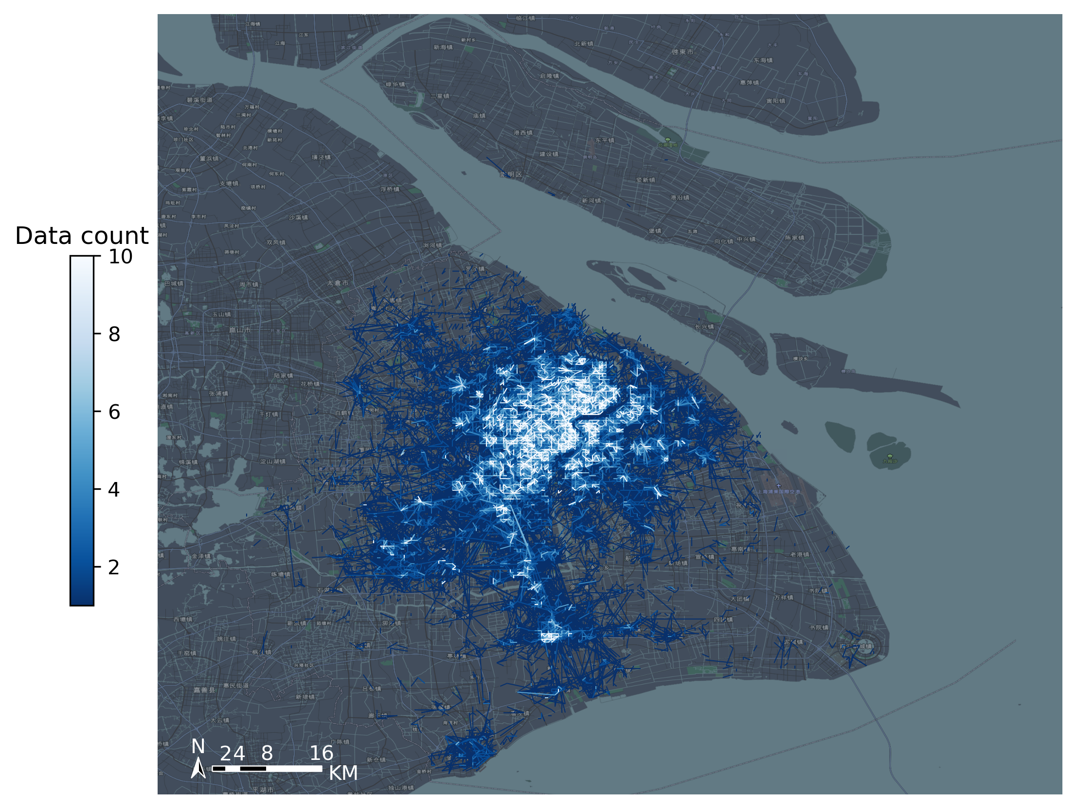
可视化OD数据
[7]:
#Create figure
import matplotlib.pyplot as plt
fig =plt.figure(1,(8,8),dpi=300)
ax =plt.subplot(111)
plt.sca(ax)

#Load basemap
tbd.plot_map(plt,bounds,zoom = 11,style = 8)

#Create colorbar
cax = plt.axes([0.05, 0.33, 0.02, 0.3])
plt.title('Data count')
plt.sca(ax)

#Plot OD
od_gdf.plot(ax = ax,column = 'count',cmap = 'Blues_r',linewidth = 0.5,vmax = 10,cax = cax,legend = True)

#Plot compass and scale
tbd.plotscale(ax,bounds = bounds,textsize = 10,compasssize = 1,textcolor = 'white',accuracy = 2000,rect = [0.06,0.03],zorder = 10)
plt.axis('off')
plt.xlim(bounds[0],bounds[2])
plt.ylim(bounds[1],bounds[3])
plt.show()
创建网络
提取节点数据
将“LONCOL”和“LATCOL”列合并到一个字段中并提取节点集
[8]:
#Combine the ``LONCOL`` and ``LATCOL`` columns into one field
od_gdf['S'] = od_gdf['SLONCOL'].astype(str) + ',' + od_gdf['SLATCOL'].astype(str)
od_gdf['E'] = od_gdf['ELONCOL'].astype(str) + ',' + od_gdf['ELATCOL'].astype(str)
#extract node set
node = set(od_gdf['S'])|set(od_gdf['E'])
node = pd.DataFrame(node)
#reindex the node
node['id'] = range(len(node))
node
[8]:
| 0 | id | |
|---|---|---|
| 0 | 164,81 | 0 |
| 1 | 71,125 | 1 |
| 2 | 102,118 | 2 |
| 3 | 125,115 | 3 |
| 4 | 143,76 | 4 |
| ... | ... | ... |
| 9806 | 98,167 | 9806 |
| 9807 | 46,130 | 9807 |
| 9808 | 118,82 | 9808 |
| 9809 | 158,57 | 9809 |
| 9810 | 104,169 | 9810 |
9811 rows × 2 columns
提取边数据
[9]:
#Merge the node information to the OD data to extract edge data.
node.columns = ['S','S_id']
od_gdf = pd.merge(od_gdf,node,on = ['S'])
node.columns = ['E','E_id']
od_gdf = pd.merge(od_gdf,node,on = ['E'])
#Extract edge data
edge = od_gdf[['S_id','E_id','count']]
edge
[9]:
| S_id | E_id | count | |
|---|---|---|---|
| 0 | 6251 | 4211 | 1 |
| 1 | 5879 | 8676 | 1 |
| 2 | 8432 | 8676 | 3 |
| 3 | 5511 | 8676 | 1 |
| 4 | 3386 | 8676 | 1 |
| ... | ... | ... | ... |
| 68468 | 5663 | 5835 | 2 |
| 68469 | 7738 | 4266 | 2 |
| 68470 | 360 | 8003 | 2 |
| 68471 | 6759 | 601 | 3 |
| 68472 | 6081 | 3107 | 3 |
68473 rows × 3 columns
创建网络
[10]:
import igraph
#Create Network
g = igraph.Graph()
#Add node
g.add_vertices(len(node))
#Add edge
g.add_edges(edge[['S_id','E_id']].values)
#Add weight
edge_weights = edge[['count']].values
for i in range(len(edge_weights)):
    g.es[i]['weight'] = edge_weights[i]
社区检测
[11]:
#Community detection
g_clustered = g.community_multilevel(weights = edge_weights, return_levels=False)
[12]:
#Modularity
g_clustered.modularity
[12]:
0.8496074605497185
[13]:
#Assign the group result to the node
node['group'] = g_clustered.membership
#rename the columns
node.columns = ['grid','node_id','group']
node
[13]:
| grid | node_id | group | |
|---|---|---|---|
| 0 | 164,81 | 0 | 0 |
| 1 | 71,125 | 1 | 1 |
| 2 | 102,118 | 2 | 2 |
| 3 | 125,115 | 3 | 3 |
| 4 | 143,76 | 4 | 4 |
| ... | ... | ... | ... |
| 9806 | 98,167 | 9806 | 9 |
| 9807 | 46,130 | 9807 | 555 |
| 9808 | 118,82 | 9808 | 6 |
| 9809 | 158,57 | 9809 | 132 |
| 9810 | 104,169 | 9810 | 86 |
9811 rows × 3 columns
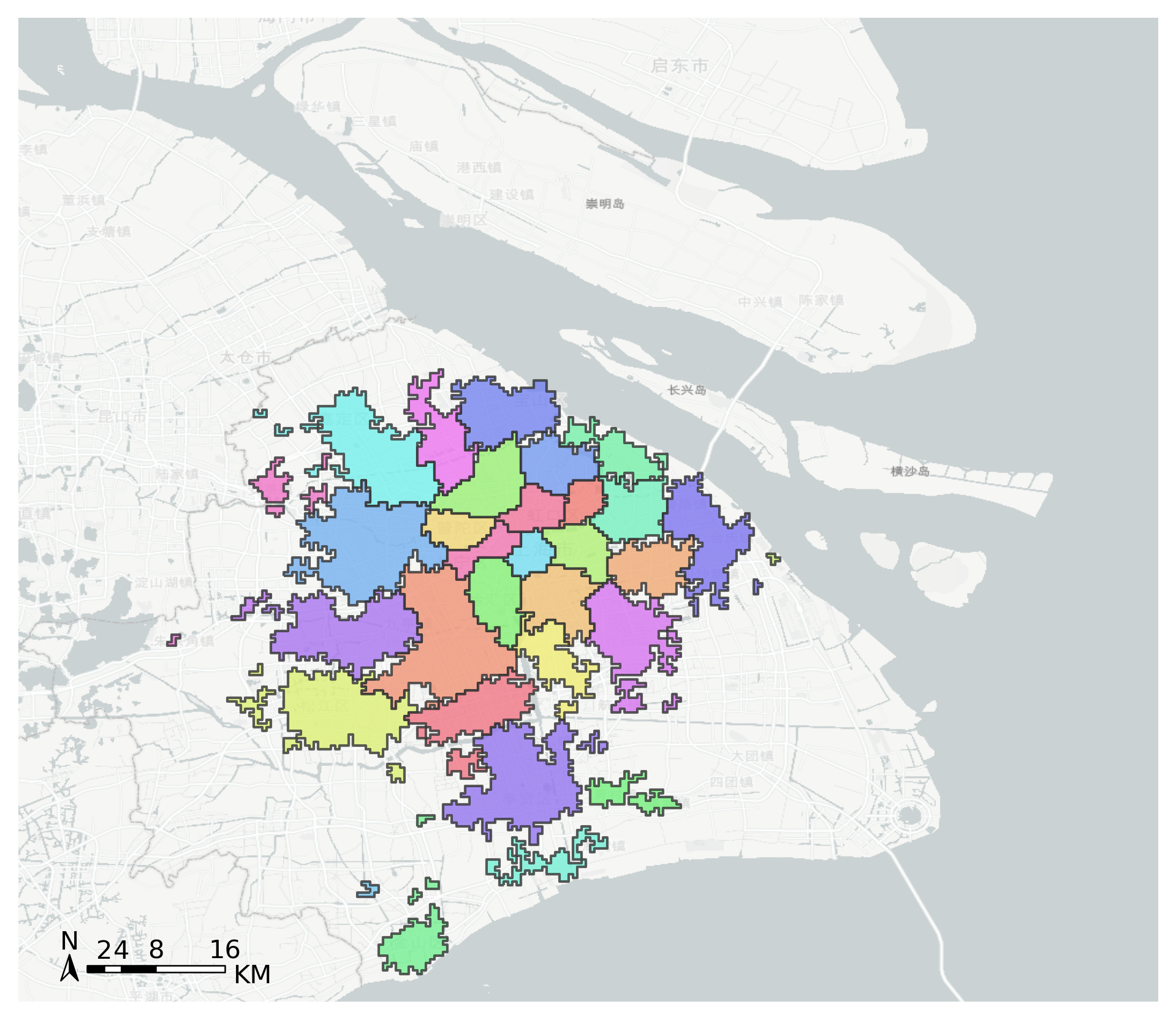
可视化社区
[14]:
#Count the number of grids per community
group = node['group'].value_counts()
#Extract communities with more than 10 grids
group = group[group>10]
#Retain only these community grids
node = node[node['group'].apply(lambda r:r in group.index)]

#Get the grid number
node['LONCOL'] = node['grid'].apply(lambda r:r.split(',')[0]).astype(int)
node['LATCOL'] = node['grid'].apply(lambda r:r.split(',')[1]).astype(int)
#Generate the geometry
node['geometry'] = tbd.gridid_to_polygon(node['LONCOL'],node['LATCOL'],params)
#Change it into GeoDataFrame
import geopandas as gpd
node = gpd.GeoDataFrame(node)
node
/var/folders/b0/q8rx9fj965b5p7yqq8zhvdx80000gn/T/ipykernel_30130/418053260.py:9: SettingWithCopyWarning:
A value is trying to be set on a copy of a slice from a DataFrame.
Try using .loc[row_indexer,col_indexer] = value instead

See the caveats in the documentation: https://pandas.pydata.org/pandas-docs/stable/user_guide/indexing.html#returning-a-view-versus-a-copy
  node['LONCOL'] = node['grid'].apply(lambda r:r.split(',')[0]).astype(int)
/var/folders/b0/q8rx9fj965b5p7yqq8zhvdx80000gn/T/ipykernel_30130/418053260.py:10: SettingWithCopyWarning:
A value is trying to be set on a copy of a slice from a DataFrame.
Try using .loc[row_indexer,col_indexer] = value instead

See the caveats in the documentation: https://pandas.pydata.org/pandas-docs/stable/user_guide/indexing.html#returning-a-view-versus-a-copy
  node['LATCOL'] = node['grid'].apply(lambda r:r.split(',')[1]).astype(int)
/var/folders/b0/q8rx9fj965b5p7yqq8zhvdx80000gn/T/ipykernel_30130/418053260.py:12: SettingWithCopyWarning:
A value is trying to be set on a copy of a slice from a DataFrame.
Try using .loc[row_indexer,col_indexer] = value instead

See the caveats in the documentation: https://pandas.pydata.org/pandas-docs/stable/user_guide/indexing.html#returning-a-view-versus-a-copy
  node['geometry'] = tbd.gridid_to_polygon(node['LONCOL'],node['LATCOL'],params)
[14]:
| grid | node_id | group | LONCOL | LATCOL | geometry | |
|---|---|---|---|---|---|---|
| 1 | 71,125 | 1 | 1 | 71 | 125 | POLYGON ((121.22089 31.22983, 121.22615 31.229... |
| 2 | 102,118 | 2 | 2 | 102 | 118 | POLYGON ((121.38398 31.19835, 121.38924 31.198... |
| 3 | 125,115 | 3 | 3 | 125 | 115 | POLYGON ((121.50498 31.18486, 121.51024 31.184... |
| 4 | 143,76 | 4 | 4 | 143 | 76 | POLYGON ((121.59967 31.00949, 121.60493 31.009... |
| 5 | 142,87 | 5 | 4 | 142 | 87 | POLYGON ((121.59441 31.05896, 121.59967 31.058... |
| ... | ... | ... | ... | ... | ... | ... |
| 9802 | 103,103 | 9802 | 8 | 103 | 103 | POLYGON ((121.38924 31.13090, 121.39450 31.130... |
| 9803 | 162,133 | 9803 | 28 | 162 | 133 | POLYGON ((121.69963 31.26580, 121.70489 31.265... |
| 9804 | 107,130 | 9804 | 41 | 107 | 130 | POLYGON ((121.41028 31.25231, 121.41554 31.252... |
| 9806 | 98,167 | 9806 | 9 | 98 | 167 | POLYGON ((121.36293 31.41868, 121.36819 31.418... |
| 9808 | 118,82 | 9808 | 6 | 118 | 82 | POLYGON ((121.46815 31.03647, 121.47341 31.036... |
8522 rows × 6 columns
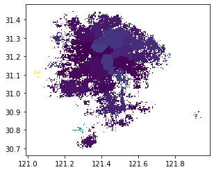
[15]:
node.plot('group')
[15]:
<AxesSubplot:>
[16]:
#Use the group column to merge polygon
node_community = tbd.merge_polygon(node,'group')
#Input polygon GeoDataFrame data, take the exterior boundary of the polygon to form a new polygon
node_community = tbd.polyon_exterior(node_community,minarea = 0.000100)
/opt/anaconda3/envs/transbigdata/lib/python3.9/site-packages/transbigdata/gisprocess.py:205: ShapelyDeprecationWarning: Iteration over multi-part geometries is deprecated and will be removed in Shapely 2.0. Use the `geoms` property to access the constituent parts of a multi-part geometry.
  for i in p:
[17]:
#Generate palette
import seaborn as sns
## l: Luminance
## s: Saturation
cmap = sns.hls_palette(n_colors=len(node_community), l=.7, s=0.8)
sns.palplot(cmap)

[19]:
#Create figure
import matplotlib.pyplot as plt
fig =plt.figure(1,(8,8),dpi=300)
ax =plt.subplot(111)
plt.sca(ax)
#Load basemap
tbd.plot_map(plt,bounds,zoom = 10,style = 6)
#Set colormap
from matplotlib.colors import ListedColormap
#Disrupting the order of the community
node_community = node_community.sample(frac=1)
#Plot community
node_community.plot(cmap = ListedColormap(cmap),ax = ax,edgecolor = '#333',alpha = 0.8)
#Add scale
tbd.plotscale(ax,bounds = bounds,textsize = 10,compasssize = 1,textcolor = 'k'
              ,accuracy = 2000,rect = [0.06,0.03],zorder = 10)
plt.axis('off')
plt.xlim(bounds[0],bounds[2])
plt.ylim(bounds[1],bounds[3])
plt.show()